In our last tutorial, “Building a Beginner-Friendly Databricks API Ingestion Pipeline with NASA API”, we successfully fetched raw daily space data from NASA’s Astronomical Picture of the Day (APOD) API and safely stored them as .jsonl files in a Databricks Volume. 

In this tutorial, we will use the modern Databricks Spark Declarative Pipelines (SDP) framework (pyspark.pipelines) to build an automated Medallion Architecture, complete with automated data ingestion, Change Data Capture (CDC) upserts, data quality expectations, and materialized business metrics.

Note: Make sure to complete the last tutorial first before proceeding.

1. Create a new ETL Pipeline

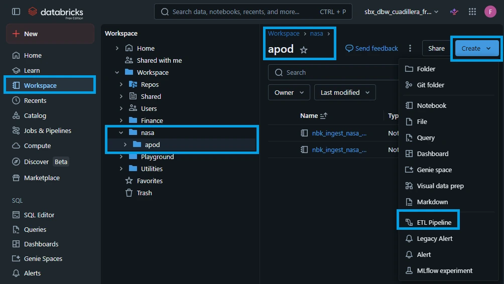
1.1. On the left-hand navigation sidebar in Databricks, click on "Workspace" and navigate to "nasa" -> "apod" folder. Click "Create" -> "ETL Pipeline"

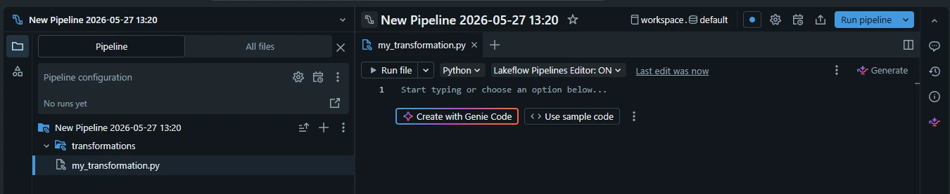
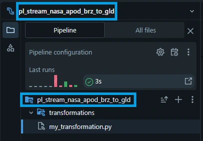
A new pipeline will be created as shown below:

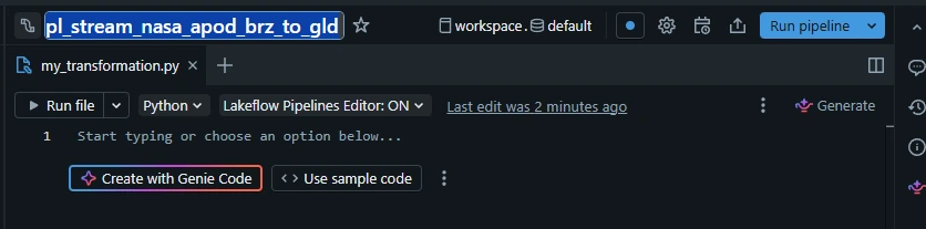
1.2. Rename the ETL pipeline. Double click the "New Pipeline ..." and type: "pl_stream_nasa_apod_brz_to_gld"

Here is the breakdown of the pl_stream_nasa_apod_brz_to_gld naming convention. It follows a modular pattern: [Type]_[Engine]_[Domain]_[Dataset]_[Source]_to_[Target].

Component	Code	Meaning
Object Type	pl	Pipeline: Distinguishes an orchestrated workflow from a table or notebook.
Execution Engine	stream	Streaming: Signals a continuous, near real-time runtime engine.
Data Domain	nasa	Data Owner: The high-level organization or system origin.
Project / Dataset	apod	Project Name: Astronomy Picture of the Day API.
Source to Target	brz_to_gld	Data Flow: Spans the entire Medallion Architecture, from Bronze (raw) to Gold (aggregated metrics).

1.3. Rename the root folder, click the kebab menu (three dots) -> click "Rename root folder": 

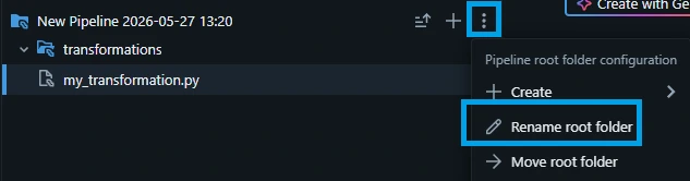
1.4. Type "pl_stream_nasa_apod_brz_to_gld" and click "OK".

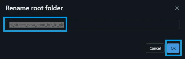
Take note that pipeline name can be different with root folder name. To avoid confusion, we will rename the root folder to match the pipeline name. 

2. Coding the Transformation Python file.

In Databricks Spark Declarative Pipelines (SDP), a transformation file is a source code file (typically in .sql or .py format) that contains the logic used to clean, filter, and enrich data within a pipeline. These files are the building blocks of an SDP project, where you "declare" the end state of your data (e.g., a cleaned table) rather than writing the step-by-step imperative code to achieve it.

Click the blank space in "my_transformation.py" paste the following python code:

from pyspark import pipelines as dp
from pyspark.sql import functions as F

"""
Bronze Layer: Ingest NASA APOD data from volume using Auto Loader
"""

@dp.table(
    name="astronomy_pictures_cdc",
    comment="Raw NASA APOD data ingested from volume using Auto Loader"
)
def astronomy_pictures_cdc():
    """
    Incrementally loads JSONL files from volume.
    Source: /Volumes/nasa_brz_sbx/apod/astronomy_pictures/
    """
    return (
        spark.readStream
        .format("cloudFiles")
        .option("cloudFiles.format", "json")
        .option("cloudFiles.inferColumnTypes", "true")
        .option("pathGlobFilter", "*.jsonl")
        .load("/Volumes/nasa_brz_sbx/apod/astronomy_pictures/")
    )

"""
Silver Layer: Clean and standardize NASA APOD data with CDC upsert logic
"""

# Preprocessing: Transform and validate data before CDC
@dp.temporary_view(name="astronomy_pictures_preprocessed")
@dp.expect_or_drop("valid_date", "date IS NOT NULL")
@dp.expect_or_drop("valid_title", "title IS NOT NULL")
@dp.expect("valid_media_type", "media_type IN ('image', 'video')")
def astronomy_pictures_preprocessed():
    """
    Transforms and validates bronze APOD data before CDC upsert
    """
    return (
        spark.readStream.table("astronomy_pictures_cdc")
        .select(
            F.col("date").cast("date").alias("date"),
            F.col("title"),
            F.col("explanation"),
            F.col("url"),
            F.col("hdurl"),
            F.col("media_type"),
            F.col("copyright"),
            F.col("service_version"),
            F.current_timestamp().alias("processed_at")
        )
    )

# Target table for CDC
dp.create_streaming_table(
    name="astronomy_pictures_cdc_clean",
    comment="Cleaned and standardized NASA APOD data with data quality checks",
    cluster_by=["date"]
)

# CDC flow: Upsert from preprocessed view to target table
dp.create_auto_cdc_flow(
    target="astronomy_pictures_cdc_clean",
    source="astronomy_pictures_preprocessed",
    keys=["date"],
    sequence_by="processed_at",
    stored_as_scd_type=1
)

"""
Gold Layer: Aggregated analytics for NASA APOD data
"""

@dp.materialized_view(
    name="astronomy_pictures_monthly_stats",
    comment="Monthly statistics of NASA APOD data"
)
def astronomy_pictures_monthly_stats():
    """
    Monthly aggregations: counts, media types, copyright distribution
    """
    return (
        spark.read.table("astronomy_pictures_cdc_clean")
        .withColumn("year_month", F.date_format("date", "yyyy-MM"))
        .groupBy("year_month")
        .agg(
            F.count("*").alias("total_apods"),
            F.sum(F.when(F.col("media_type") == "image", 1).otherwise(0)).alias("image_count"),
            F.sum(F.when(F.col("media_type") == "video", 1).otherwise(0)).alias("video_count"),
            F.sum(F.when(F.col("copyright").isNotNull(), 1).otherwise(0)).alias("copyrighted_count"),
            F.sum(F.when(F.col("copyright").isNull(), 1).otherwise(0)).alias("public_domain_count"),
            F.min("date").alias("first_date"),
            F.max("date").alias("last_date")
        )
        .orderBy("year_month")
    )

This pipeline implements a streaming Medallion Architecture using Databricks Spark Declarative Pipelines (SDP). The framework replaces traditional manual Spark Structured Streaming orchestration (managing .writeStream(), checkpoints, and explicit trigger intervals) with a declarative model. The engine builds a directed acyclic graph (DAG) and natively manages state management, checkpoint transactions, and optimization schedules.

2.1. Setup the environment for building Spark Declarative Pipelines (SDP)

from pyspark import pipelines as dp
from pyspark.sql import functions as F

This code imports tools to build managed data pipelines and transform data in PySpark.

• from pyspark import pipelines as dp: Imports Spark Declarative Pipelines. It lets you define tables, materialized views, and data quality rules using decorators.
• from pyspark.sql import functions as F: Imports standard Spark SQL functions (like sum, count, or col). The F alias avoids naming conflicts with Python's built-in functions.

2.2. Bronze Ingestion Layer: Idempotent File Streaming

@dp.table(
    name="astronomy_pictures_cdc",
    comment="Raw NASA APOD data ingested from volume using Auto Loader"
)
def astronomy_pictures_cdc():
    return (
        spark.readStream
        .format("cloudFiles")
        .option("cloudFiles.format", "json")
        .option("cloudFiles.inferColumnTypes", "true")
        .option("pathGlobFilter", "*.jsonl")
        .load("/Volumes/nasa_brz_sbx/apod/astronomy_pictures/")
    )

Technical Mechanics

• @dp.table Registration: This decorator tells the pipeline manager to provision and manage a persistent Streaming Table. Unlike a standard Delta table, a Streaming Table guarantees incremental processing semantics by default.

• Auto Loader (cloudFiles): Natively tracks newly arrived files in the Unity Catalog Volume source path. It scales efficiently by avoiding expensive directory listing operations, using optimized file notifications or incremental directory listing hooks instead.

• Schema Inference & Evolution: Setting cloudFiles.inferColumnTypes to true causes the engine to automatically sample raw .jsonl files to determine data types. It stores this schema metadata internally, preventing stream failure if a new field is introduced by the API.

• Transactional State Management: The runtime engine manages the checkpoint location under the hood. It ensures exactly-once processing guarantees by logging successfully processed files into its transaction log, making file discovery completely idempotent.

2.3. Silver Layer: Data Quality Governance & CDC Merge

The Silver Layer is broken into three distinct execution phases: preprocessing/validation, target table initialization, and an automated Change Data Capture (CDC) engine merge.

2.3.1. Phase A: Preprocessing and Quality Expectations

@dp.temporary_view(name="astronomy_pictures_preprocessed")
@dp.expect_or_drop("valid_date", "date IS NOT NULL")
@dp.expect_or_drop("valid_title", "title IS NOT NULL")
@dp.expect("valid_media_type", "media_type IN ('image', 'video')")
def astronomy_pictures_preprocessed():
    return (
        spark.readStream.table("astronomy_pictures_cdc")
        .select(
            F.col("date").cast("date").alias("date"),
            F.col("title"),
            F.col("explanation"),
            F.col("url"),
            F.col("hdurl"),
            F.col("media_type"),
            F.col("copyright"),
            F.col("service_version"),
            F.current_timestamp().alias("processed_at")
        )
    )

• @dp.temporary_view: This registers an in-memory logical view within the pipeline DAG. No data is physically serialized or persisted to disk at this step. It acts as an ephemeral processing node in the streaming lineage.

• Data Quality Expectations:

  • @dp.expect_or_drop: Enforces hard validation rules. If a record violates the SQL expression "date IS NOT NULL" or "title IS NOT NULL", the entire row is dropped from the active stream and recorded as a failed metric in the pipeline event log.

  • @dp.expect: Implements a soft rule. If a record contains a media_type other than 'image' or 'video', the row is still processed, but the event log registers a quality metric alert.

• dp.read_stream() Semantics: Passing spark.readStream.table() into the pipeline forces Spark to read the transaction log of the Bronze table incrementally, ensuring only newly appended blocks are passed downstream.

2.3.2. Phase B: Target Table Initialization

dp.create_streaming_table(
    name="astronomy_pictures_cdc_clean",
    comment="Cleaned and standardized NASA APOD data with data quality checks",
    cluster_by=["date"]
)

• Liquid Clustering (cluster_by): This allocates physical storage blocks based on the date key. Liquid clustering replaces traditional hard-partitioning rules with a flexible layout that dynamically handles data skew and speeds up query execution for time-series lookups on downstream tables.

2.3.3. Phase C: Change Data Capture (SCD Type 1 Upsert)

dp.create_auto_cdc_flow(
    target="astronomy_pictures_cdc_clean",
    source="astronomy_pictures_preprocessed",
    keys=["date"],
    sequence_by="processed_at",
    stored_as_scd_type=1
)

• Stateful Deduplication: Under standard Structured Streaming, handling updates requires complex watermarking and a manual foreachBatch(merge...) routine. dp.create_auto_cdc_flow abstracts this complexity entirely.

• keys and sequence_by: The engine checks incoming records against the target table using date as the primary key. If a record matches an existing date, the engine compares the processed_at timestamps. The record with the higher value wins, ensuring out-of-order API updates are resolved correctly.

• stored_as_scd_type=1: This sets an overwrite strategy (Slowly Changing Dimension Type 1). Existing rows matching the target key are updated in place, while entirely new dates are appended.

2.4. Gold Layer: Incremental Materialized Aggregations

@dp.materialized_view(
    name="astronomy_pictures_monthly_stats",
    comment="Monthly statistics of NASA APOD data"
)
def astronomy_pictures_monthly_stats():
    return (
        spark.read.table("astronomy_pictures_cdc_clean")
        .withColumn("year_month", F.date_format("date", "yyyy-MM"))
        .groupBy("year_month")
        .agg(
            F.count("*").alias("total_apods"),
            F.sum(F.when(F.col("media_type") == "image", 1).otherwise(0)).alias("image_count"),
            F.sum(F.when(F.col("media_type") == "video", 1).otherwise(0)).alias("video_count"),
            F.sum(F.when(F.col("copyright").isNotNull(), 1).otherwise(0)).alias("copyrighted_count"),
            F.sum(F.when(F.col("copyright").isNull(), 1).otherwise(0)).alias("public_domain_count"),
            F.min("date").alias("first_date"),
            F.max("date").alias("last_date")
        )
        .orderBy("year_month")
    )

Technical Mechanics

• @dp.materialized_view: Unlike streaming tables that ingest appends incrementally, a Materialized View is designed for queryable aggregates. The framework determines the upstream changes and computes updates to refresh the view automatically.

• spark.read.table() Semantics: Notice the switch to a standard batch read (spark.read.table) instead of readStream. The framework reads the pre-computed state from the Silver table. During execution, the pipeline engine optimizes this process under the hood, refreshing only the modified data groups (months) rather than scanning the entire historical table.

• Analytical Matrix Optimization: The groupBy("year_month") operation aggregates metrics into high-performance business lookups. When consumer tools query this view, Databricks reads directly from the pre-computed snapshot table, dropping analytical query times down to milliseconds.

2. Validating Your Pipeline with a Dry Run

Before deploying a streaming data pipeline to production, it is a data engineering best practice to validate the structural integrity of your code. Databricks Spark Declarative Pipelines include a built-in Dry Run feature.

By definition, a Dry Run checks all definitions, schema types, data constraints, and dataset references across your entire pipeline DAG without provisioning production compute clusters, initializing cloud files tracking, or creating/updating any physical target tables.

This makes it an incredibly fast, zero-cost mechanism for developing, local testing, and debugging your ETL code.

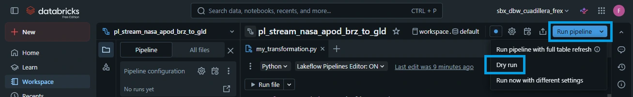
1. 2.1. In the top-right corner, click the dropdown arrow next to the "Run pipeline" button.

2. 2.2. Select "Dry run".

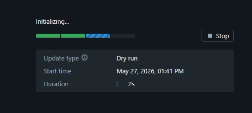
3. 2.3. Wait for the Dry run to finish.

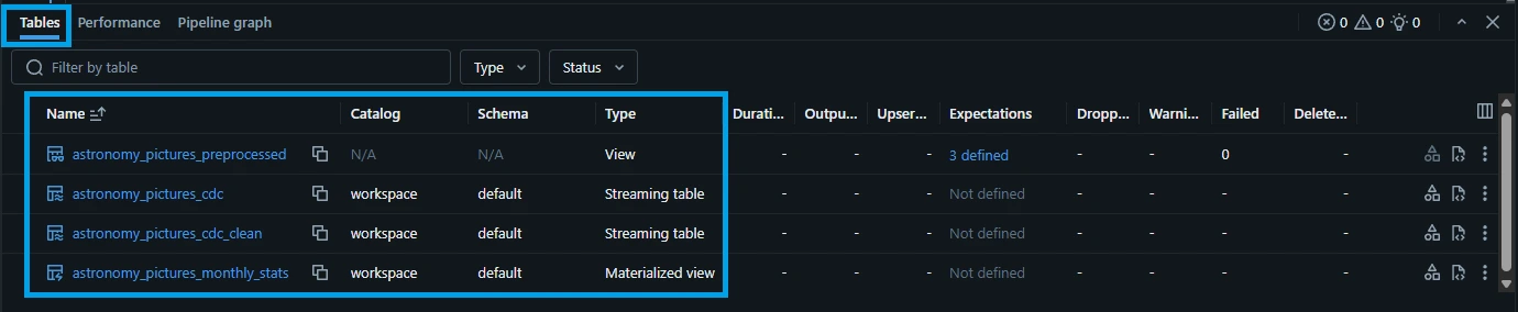
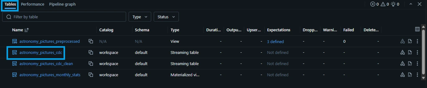
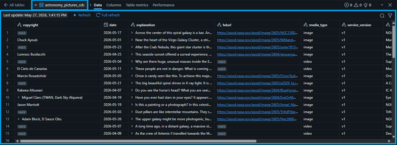
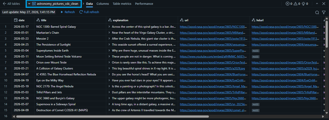
4. 2.4. Once the "Dry Run" finishes, we can see that the tables and views has been created temporarily to verify the correctness of the code. Click the "astronomy_pictures_cdc" (bronze table) to preview the data.

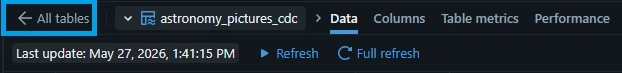
5. 2.5. Let's check the other tables. Click the "<- All tables" button. Click the "astronomy_pictures_cdc_clean" (silver table).

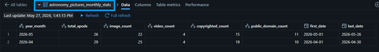
6. 2.6. Repeat the same steps to check the "astronomy_pictures_monthly_stats" (gold table).
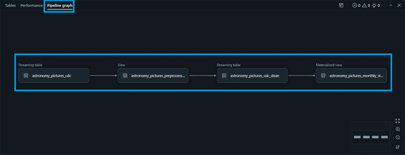
7. 2.7. Let's check the "Pipeline graph". Click the "Pipeline graph" button. It is a visual representation of your data transformation workflow, specifically known as a directed acyclic graph (DAG).

3. Run the pipeline

3.1. Running a pipeline means telling Databricks to automatically build, update, and manage your data tables based on the rules (Python/SQL) you already defined.

Note: Ideally, we can design the pipeline to create the bronze, silver, and gold tables across different catalogs by explicitly defining the three level namespace within the decorator. For example: 
* name = "nasa_brz_sbx.apod.astronomy_pictures_cdc"
* name = "nasa_slv_sbx.apod.astronomy_pictures_cdc_clean"
* name = "nasa_gld_sbx.apod.astronomy_pictures_monthly_stats"

This is not possible in Databricks Free Edition which is a known limitation. Attempting this will throw an error: "PERMISSION_DENIED: Can not move tables across arclight catalogs". Refer to https://community.databricks.com/t5/databricks-free-edition-help/unity-catalog-error-permission-denied-can-not-move-tables-across/td-p/149229 for more details.

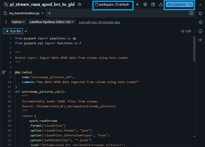
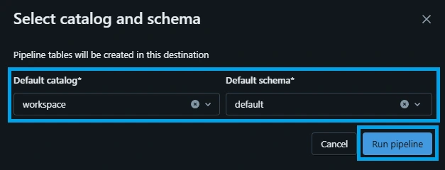
3.2. Select the default catalog and schema and click "Run pipeline".

• Default catalog: workspace
• Default schema: default

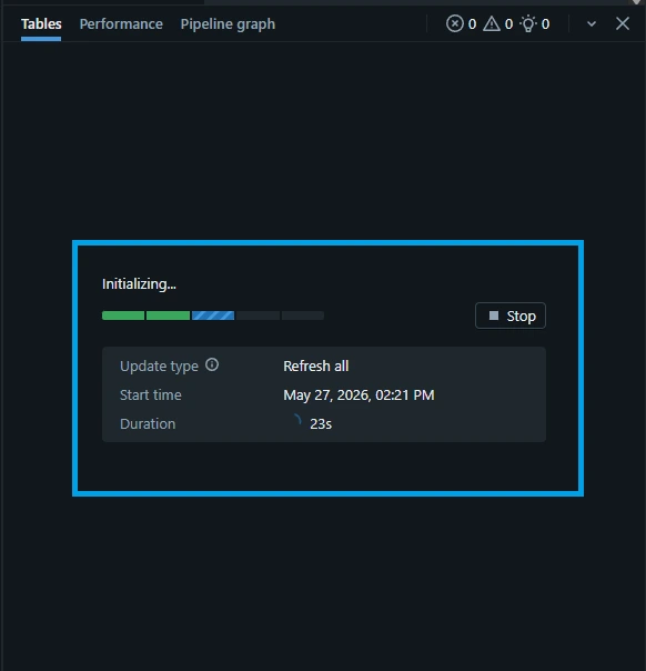
3.3. Wait for the pipeline run to finish.

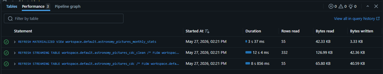
3.4. Once finished, check the performance tab. Click the "Performance" tab. In this tab, you can see the actual SQL statements equivalent of the Python code that is being executed during the process.

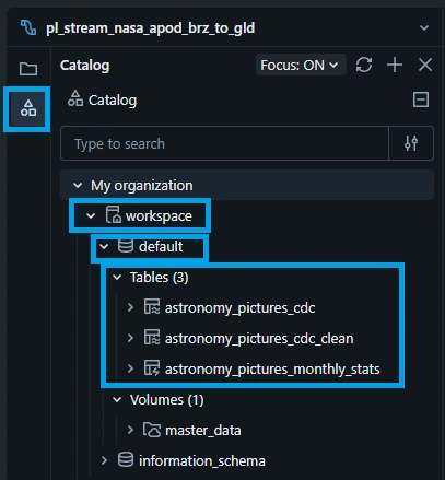
3.5. On the left side, click the catalog icon and drill down to "workspace -> default -> Tables". You can see that the tables are automatically created by the pipeline.

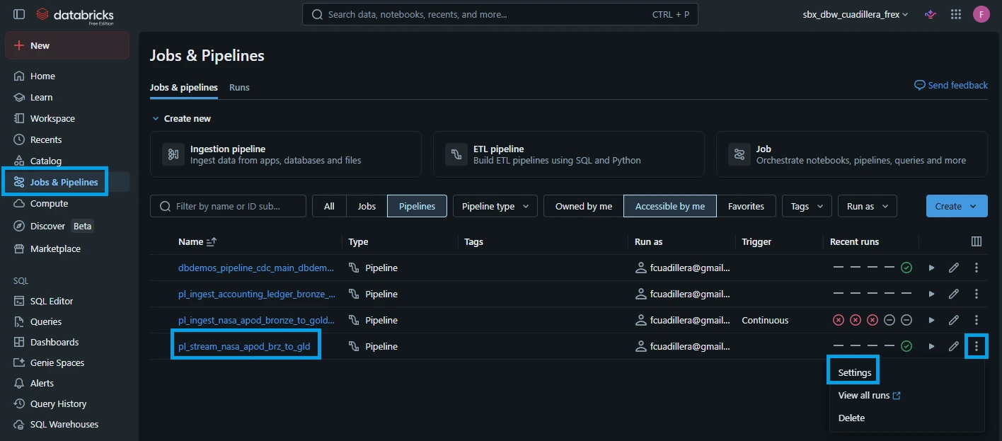
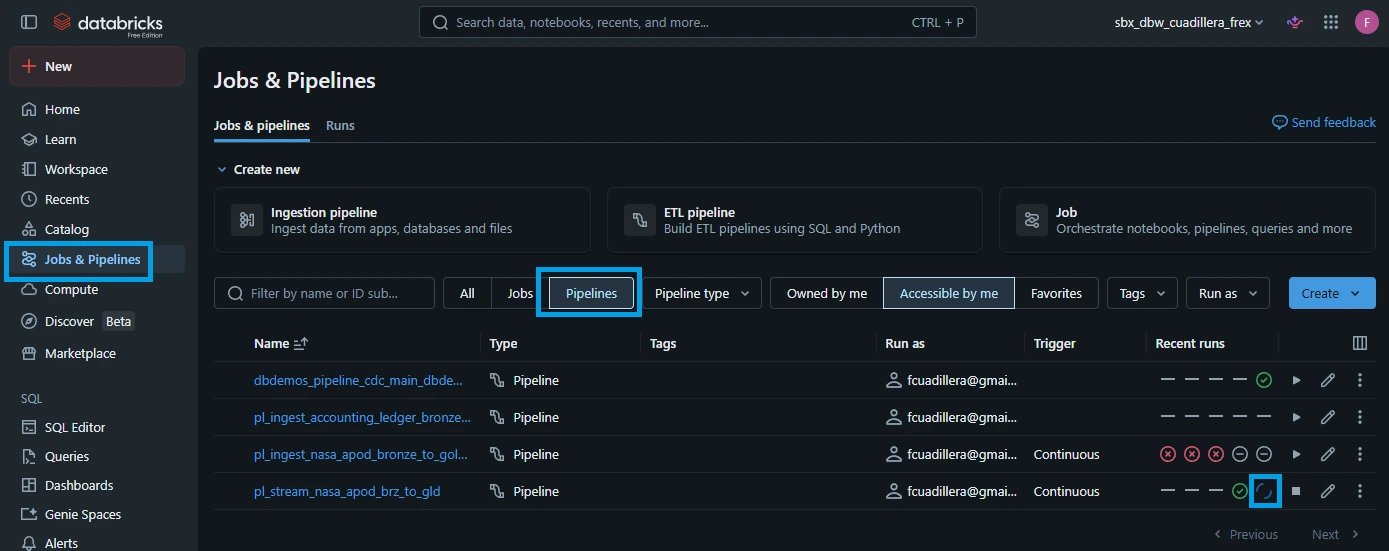
3.6. We want the streaming pipeline to run continuously. On the left-hand navigation sidebar in Databricks, click "Jobs & Pipelines" look for the "pl_stream_nasa_apod_brz_to_gld" pipeline. Click the kebab button on the right side and click "settings".

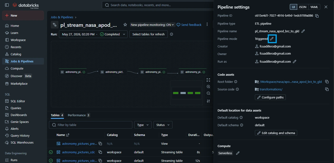
3.7. On the "Pipeline settings" pane shown on the right, look for the "Pipeline mode" and click the pencil icon to edit.

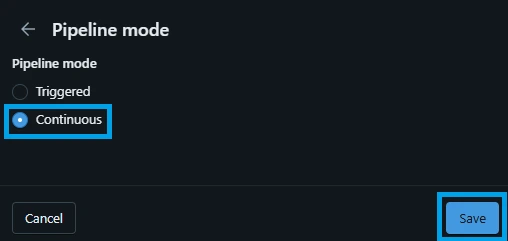
3.8. Select "Continuous" and click "Save".

3.9. Go back to the "Jobs & Pipelines" and you can see that the pipeline runs continuously with the blue circling icon.

4. Backfilling NASA APOD data to start the streaming pipeline

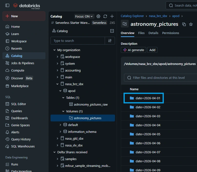
4.1. Lets put the streaming pipeline in action. From the previous tutorial, we backfilled April 2026 data. To verify the oldest APOD available, go to "Catalog -> nasa_brz_sbx -> Volumes -> astronomy_pictures". Based on the screenshot below, the oldest file is "date=2026-04-01".

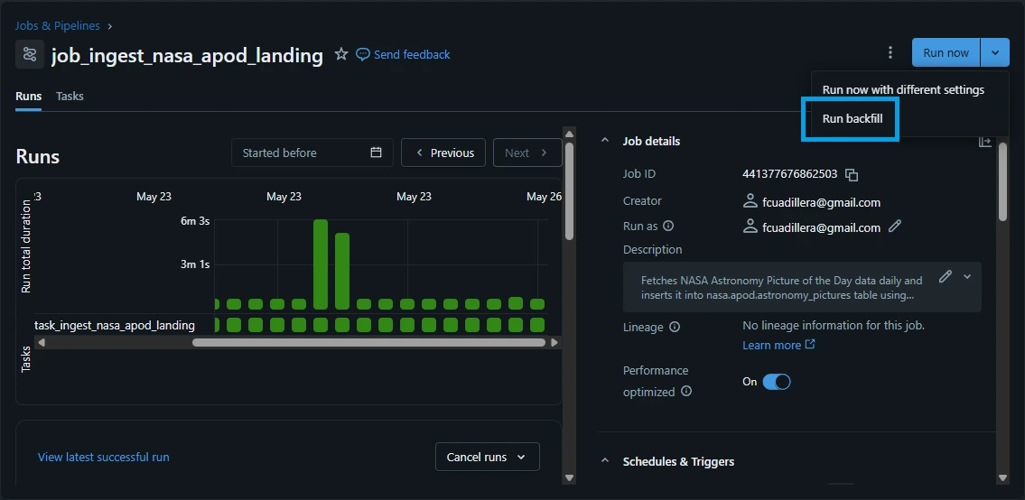
4.2. Trigger a backfill job. Go to "Jobs & Pipelines" -> "job_ingest_nasa_apod_landing".

4.3. On the right top corner, click the down arrow icon beside "Run now" button, and select "Run backfill".

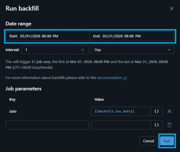
4.4. Select the "Date range" to March 2026.

• Start: 03/01/2026 08:00 PM
• End: 03/31/2026 08:00 PM

Click "Run".

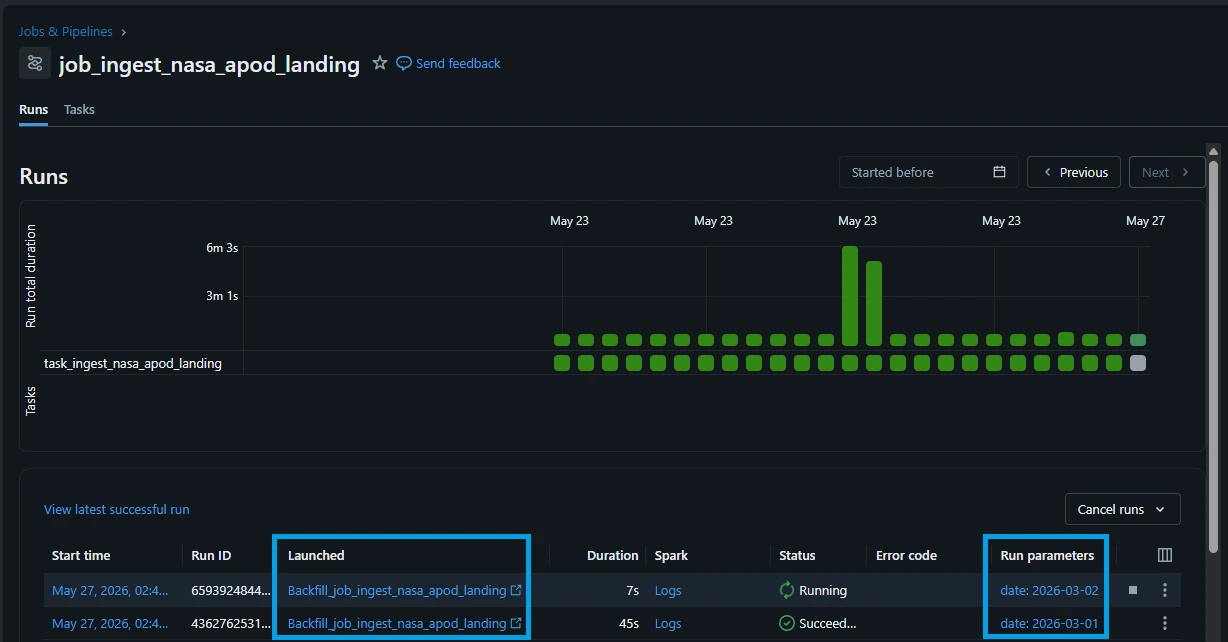
You can see that the backfill job has been started.

4.5. Go back to "Jobs & Pipelines" -> "pl_stream_nasa_apod_brz_to_gld". Click the blue circle on the "Recent runs".

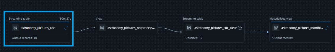
Lets visualize what happens within the streaming pipeline.

Step 1 - Streaming table: astronomy_pictures_cdc (bronze layer)

This process loads any newly arrived jsonl files in the volume that was retrieved by the backfill job.

Step 2 - View: astronomy_pictures_preprocessed & Streaming table: astronomy_pictures_cdc_clean (silver layer)

The data quality expectations are being evaluated against the temporary view before loading the valid records into the silver table.

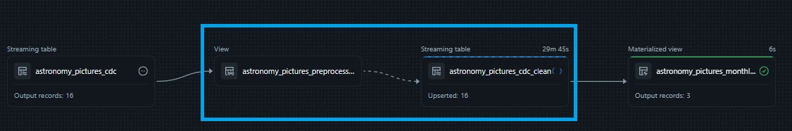
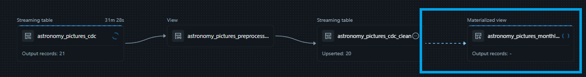
Step 3 - Materialized View: astronomy_pictures_monthly_stats (gold layer)

The last step is simply updating the materialized view.

A materialized view is a database object that precomputes and physically stores the results of a query as a table.

In Databricks, Materialized Views (MVs) are often preferred for the Gold layer over traditional "normal" Delta tables (created via INSERT/MERGE) because they provide automated, incremental, and highly performant data transformation, specifically optimized for BI consumption. While normal tables require manual management of MERGE logic and orchestrating tasks, materialized views handle these complexities automatically within the Unity Catalog, making them better suited for the high-performance needs of the final consumption layer.

Interestingly, you can see that the Step 1 already started processing the next available APOD data while the materialized view is being updated it is because Spark Declarative Pipelines decouple each layer using independent streaming states and materialized view refresh mechanics, the pipeline operates like a factory assembly line. It does not need to pause ingestion just because a downstream layer is running a complex aggregation.

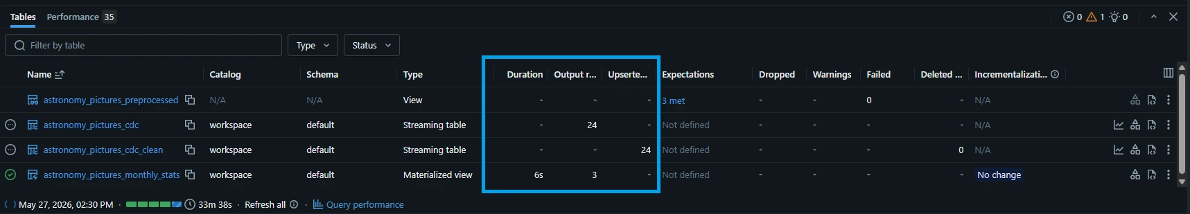
We can also see that total output records and upserted records during the run at the "Tables" tab below.

5. The "30 vs. 29" Mystery (Streaming vs. File-Triggered Ingestion)

While developing, you might notice a fascinating data discrepancy:

• job_ingest_nasa_apod_raw: run status is pending
• pl_stream_nasa_apod_brz_to_gld: run status is continuous.

Go to SQL editor and execute the following SQL queries:

select count(*) from workspace.default.astronomy_pictures_cdc where date < '2026-04-01';

select count(*) from nasa_brz_sbx.apod.astronomy_pictures_raw where date < '2026-04-01';

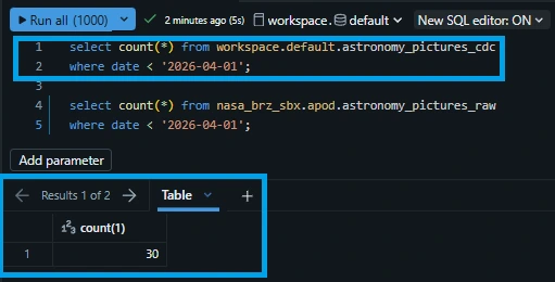
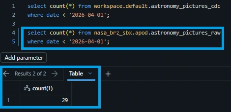
Why is the streaming table ahead by one record? This perfectly demonstrates the speed advantage of a live streaming pipeline over traditional file-arrival batch triggers.

5.1. The Technical Reason: Ingestion Race Conditions

• The Streaming Table (Continuous Latency): The Bronze table uses Auto Loader. In a continuous state, Auto Loader detects files the microsecond bytes hit the Volume. It aggressively streams and commits new records in near real-time—often before the upstream API extraction script has fully finished closing out the upload batch.

• The Raw Table (Post-Arrival Triggers): The raw target table relies on an orchestrated batch job or a file-arrival trigger. This process must wait until the file upload is 100% complete, wake up a cluster, scan the directory, and then execute the append.

The streaming pipeline is simply faster. It grabbed and committed the 30th record while the file-arrival trigger was still initializing, proving that declarative streaming gets insights to your analysts minutes ahead of traditional batch schedules.

6. Conclusion

6.1. Spark Declarative Pipelines vs. Custom Spark Jobs

Choosing between Databricks Spark Declarative Pipelines (SDP) and a traditional Custom Spark Job comes down to choosing automation over raw configuration.

Spark Declarative Pipelines (SDP)

• The Verdict: Best for standardizing structured data engineering practices across a team.

• Why: By declaring what data targets you want rather than how to build them, the engine automatically handles checkpoint transactions, schema evolution, and optimal cloud hardware scaling. Features like built-in Data Quality Expectations and automated CDC flows (dp.create_auto_cdc_flow) eliminate hundreds of lines of complex boilerplate code, making code maintenance incredibly low-effort.

Custom Spark Jobs

• The Verdict: Reserved for highly specialized edge cases.

• Why: Custom jobs (using manual .writeStream() loops) are only necessary if your pipeline requires low-level, hyper-specific control over infrastructure, non-standard stateful streaming operations, or integration with external systems that sit completely outside of the Unity Catalog governance layer.

6.2. Continuous Streaming vs. File Arrival Triggers

The decision between a Continuous Stream and a File Arrival Trigger determines how fast your business can react to incoming insights.

Continuous Streaming

• The Verdict: The choice for modern, responsive data platforms.

• Why: As demonstrated by the "30 vs. 29" mystery, continuous streaming combined with Auto Loader offers sub-second file discovery. It removes the operational overhead of spinning up clusters and checking directory folders on a rigid timer. Furthermore, its pipelined architecture allows the Bronze layer to ingest new files concurrently while downstream Gold layers compute older data aggregates.

File Arrival Triggers

• The Verdict: Ideal for cost-optimized, low-frequency batch patterns.

• Why: If your upstream API or source system only updates once a day or once a week, a continuous cluster wasting idle compute time makes no financial sense. File arrival triggers excel here: they allow you to keep compute costs at absolute zero until the file upload is 100% finished, at which point the infrastructure wakes up, processes the data as an efficient micro-batch, and safely shuts back down.

6.3. Final Synthesis

For the NASA APOD pipeline, the combination of Spark Declarative Pipelines running on a Continuous Stream is the superior architectural pattern. It provides a self-healing, self-optimizing system that processes cosmic data the moment it hits cloud storage, delivering clean and aggregated business metrics to your data analysts with zero operational friction.

#Data #DataEngineer #DataEngineering #Databricks #NASA