Building a Beginner-Friendly Databricks API Ingestion Pipeline with NASA API

Learn API ingestion, storage design, and orchestration using free NASA datasets.

May 19, 2026 by

Frex Cuadillera

1. Introduction

1.1. Project overview

This guide demonstrates fundamental data engineering concepts in Databricks using NASA’s free Astronomy Picture of the Day (APOD) API as the data source. The guide walks through the end-to-end process of consuming REST APIs, storing raw data, configuring cloud storage structures, and automating ingestion process through scheduled and event-driven jobs.

By the end, readers will gain hands-on exposure to core data engineering practices including API ingestion, file-based processing, orchestration, and building a simple medallion-style architecture within Databricks.

1.2. Architecture diagram

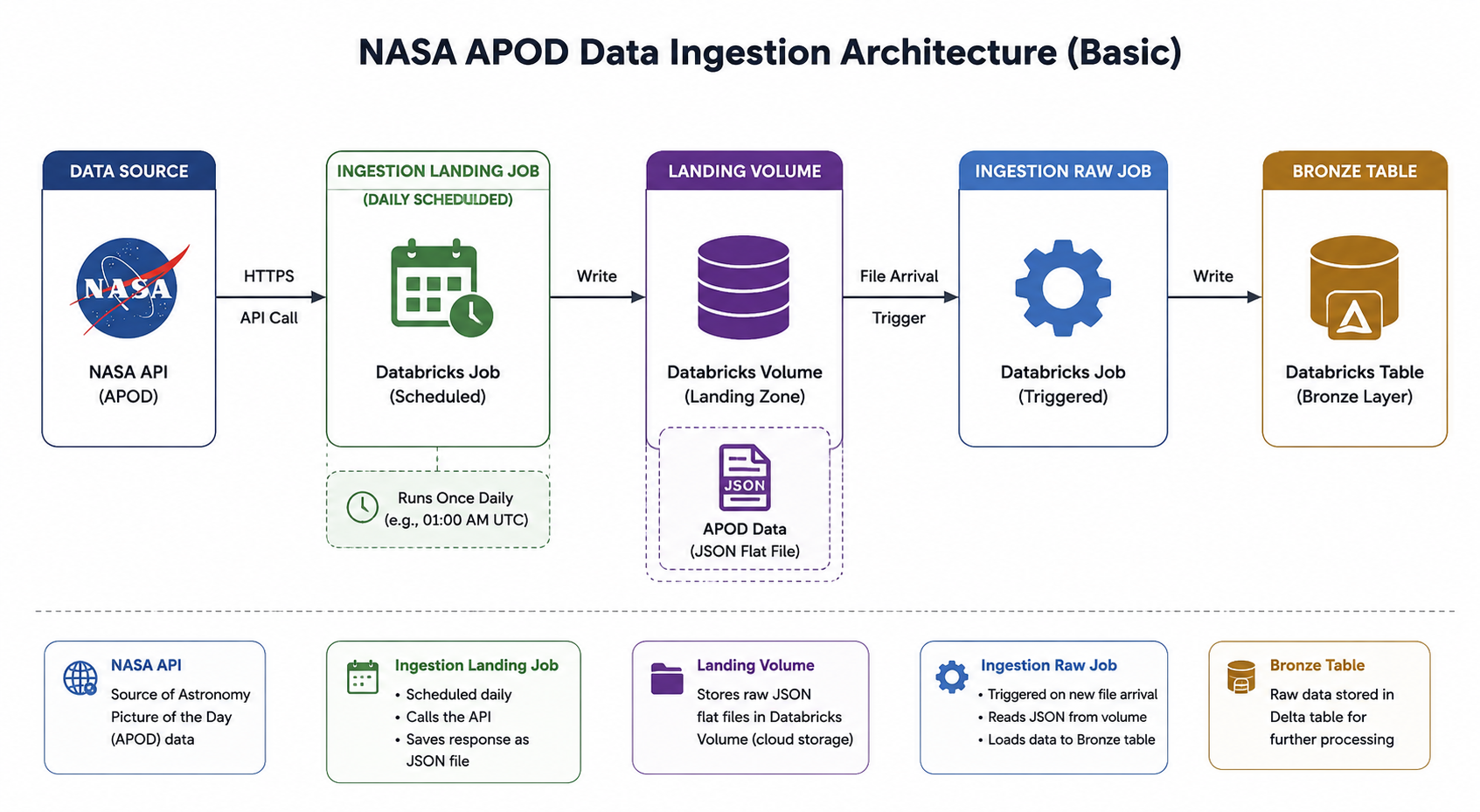
The diagram illustrates a simple end-to-end Databricks data ingestion pipeline using NASA’s APOD API as the source.

It starts with the NASA API, where data is pulled through an HTTPS request. A scheduled Databricks ingestion job runs daily to extract this data and writes it as JSON flat files into a Databricks Volume, acting as the landing zone. Once a new file arrives, a trigger-based ingestion job is activated, which reads the landed JSON data and loads it into a Bronze Delta table for structured storage and downstream processing.

Overall, the flow demonstrates a basic ingestion job commonly used by medallion-style setup with both scheduled and event-driven ingestion patterns.

2. Registering for a NASA API Key

Getting a NASA API key is incredibly straightforward and takes less than a minute. NASA uses an instant approval system, so you don't have to wait around for a verification process to wrap up.

2.1. Registration Steps

Here is exactly how to get your key and make your first data request:

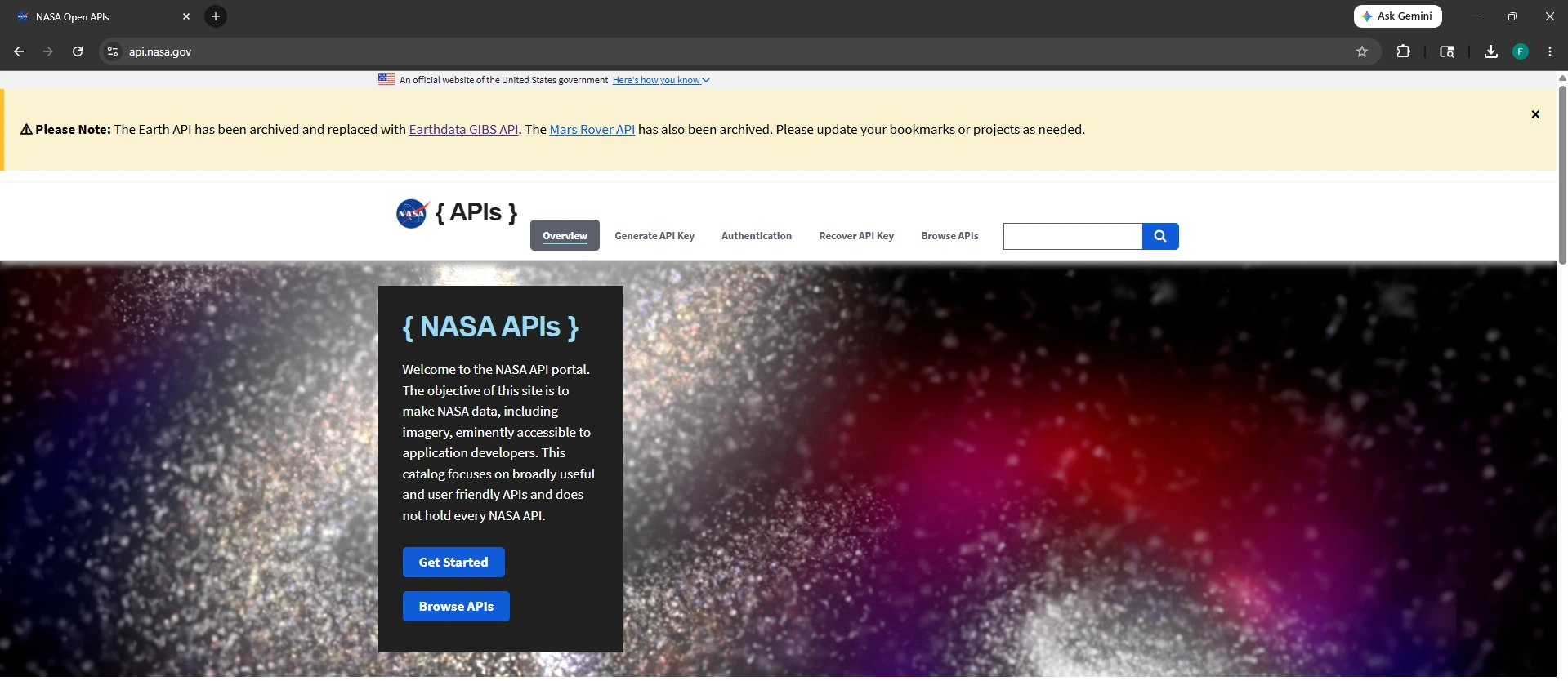
1.Visit the NASA API Portal:

Open your browser and navigate directly to the official portal at api.nasa.gov.

2.Fill out the registration form: (Requires basic info.)

Scroll down slightly on the homepage to find the Generate API Key sign-up form. You only need to provide:

First Name
Last Name
Email Address
How will you use the APIs? (Optional — you can leave this blank if you are just testing it out)

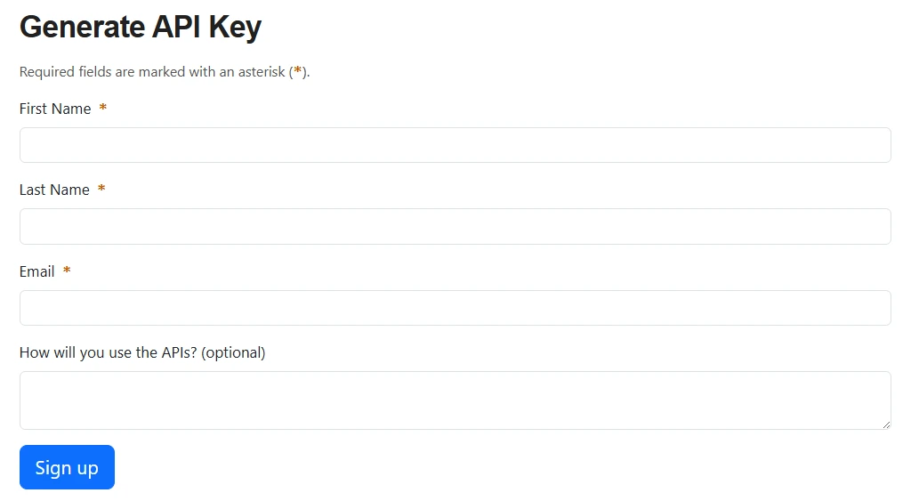
3.Submit and copy your key: Instant approval.

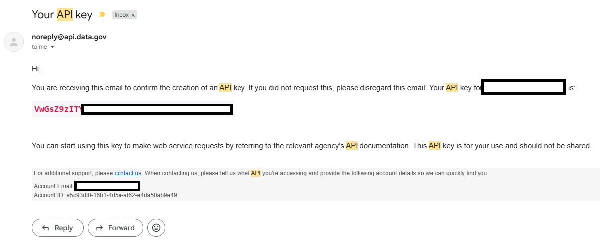
Click the Signup button. The webpage will refresh immediately and display your brand-new unique API key on the screen. NASA will also email a copy of this key to you for your records.

2.2. Testing Your Key

NASA APIs use basic query parameters for authentication. To make sure your key is active, you can test it directly in your browser using the Astronomy Picture of the Day (APOD) endpoint.

Replace YOUR_API_KEY in the URL below with the actual key you just generated, and paste it into your browser's address bar:

https://api.nasa.gov/planetary/apod?api_key=YOUR_API_KEY&date=YYYY-MM-DD

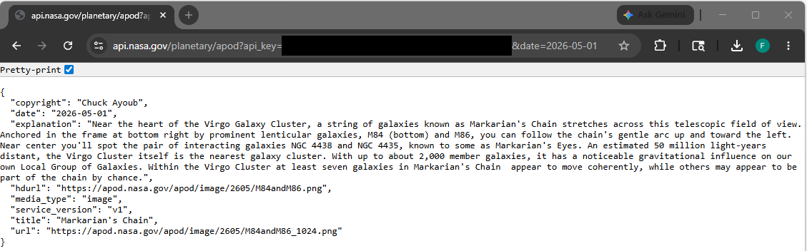
If it works, you will receive a clean JSON response containing metadata about today's space imagery, including an explanation text and a direct URL to the photo.

⚠️ Keep in mind the API Rate Limits:
Registered Key: Gives you up to 1,000 requests per hour.

3. Exploring NASA APIs Through Documentation

Before writing a single line of code, it helps to understand that NASA doesn’t just offer one API, it provides a gateway to dozens of distinct repositories. Depending on whether your project requires high-definition imagery, historical planet data, or real-time tracking, you will want to select the tool built for the job.

3.1. Five Datasets to Build With

Dataset	Core Focus	Visual vs. Text	Great For
APOD	Daily astronomical media & professional insights	High (Images/Videos)	Beginner scripts, daily notifications
Mars Rover Photos	Raw field telemetry from Martian explorers	High (Raw Mast/Nav Cams)	Filtering apps, custom galleries
NeoWs	Orbital tracking of near-Earth asteroids	Low (Pure JSON Metrics)	Data visualizations, charts, trackers
Earth Imagery	Landsat spatial data mapped to coordinates	High (Satellite views)	Geographic timelines, climate tracking
EPIC	Full-disc, live color imagery of Earth	High (Global view)	Dynamic wallpapers, rotation animations

4. Testing the APOD API in Browser & Understanding Parameters

APOD (Astronomy Picture of the Day). The most popular starting point. It fetches a daily cosmic image or video alongside commentary written by a professional astronomer.

Endpoint: GET [https://api.nasa.gov/planetary/apod](https://api.nasa.gov/planetary/apod)
Key Parameters:
- date (string, YYYY-MM-DD): The specific day you want to pull.
- count (integer): Returns a specified number of randomly chosen images (cannot be combined with dates).
- thumbs (boolean): Set to true to return a video thumbnail URL if the asset isn't a static image.
Response Format: A flat JSON object containing url, hdurl, title, explanation, and media_type.
Prime Use Case: Building a daily automation workflow that texts, emails, or tweets a beautiful new space photo every morning.

Example API response:

{
  "copyright": "Chuck Ayoub",
  "date": "2026-05-01",
  "explanation": "Near the heart of the Virgo Galaxy Cluster, a string of galaxies known as Markarian's Chain stretches across this telescopic field of view. Anchored in the frame at bottom right by prominent lenticular galaxies, M84 (bottom) and M86, you can follow the chain's gentle arc up and toward the left. Near center you'll spot the pair of interacting galaxies NGC 4438 and NGC 4435, known to some as Markarian's Eyes. An estimated 50 million light-years distant, the Virgo Cluster itself is the nearest galaxy cluster. With up to about 2,000 member galaxies, it has a noticeable gravitational influence on our own Local Group of Galaxies. Within the Virgo Cluster at least seven galaxies in Markarian's Chain  appear to move coherently, while others may appear to be part of the chain by chance.",
  "hdurl": "https://apod.nasa.gov/apod/image/2605/M84andM86.png",
  "media_type": "image",
  "service_version": "v1",
  "title": "Markarian's Chain",
  "url": "https://apod.nasa.gov/apod/image/2605/M84andM86_1024.png"

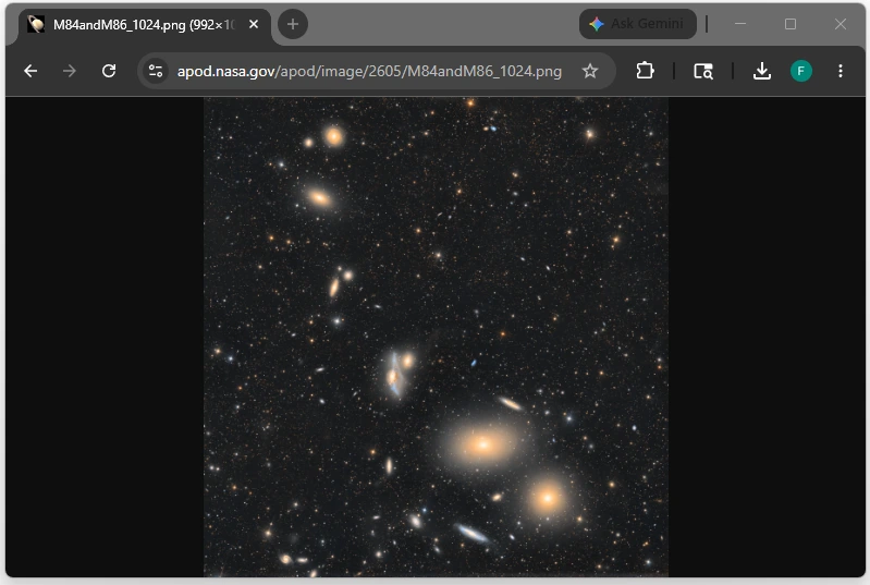
Example image:

5. Designing the Databricks Environment

In this demo, you need to have a Databricks free edition workspace.

Refer to this article before proceeding on the next steps: https://docs.databricks.com/aws/en/getting-started/free-edition

This section teaches you on how to provision Databricks objects required to setup the environment:

5.1. Catalog

In Databricks Unity Catalog (their unified data governance tool), a Catalog is the top-level container for data asset organization below the metastore itself. It implements a standard three-tier namespace: catalog.schema.table.

Think of a catalog as a massive storage bucket that isolates data by environment, team, or business unit. By isolating your data at the catalog level, you can enforce security permissions, track data lineage, and share assets without risking data leaking across environments.

5.1.1. The Breakdown of Your Catalog Name: nasa_brz_sbx

You are utilizing a fantastic enterprise naming convention here by weaving together your data source, architectural layer, and environment:

nasa: The data source prefix (identifies this belongs to your NASA API pipeline).
brz: The Bronze layer from the Medallion Architecture. This represents raw, appended data directly ingested from your NASA API payloads (often messy JSON or raw tables).
sbx: The Sandbox environment. This isolates experimental or exploratory work away from your core development (dev), quality assurance (qa), and production (prod) systems.

Note on Naming Conventions: While we are building nasa_brz_sbx today, you can easily adapt this guide to fit whatever specific enterprise naming framework your team prefers (e.g., sbx_bronze_nasa or nasa_bronze_sandbox).

5.1.2. Step-by-Step Guide: Creating Your Catalog

To create a catalog, you will need Metastore Admin privileges or a role that has the explicit CREATE CATALOG privilege on your Unity Catalog metastore.

You can create this catalog via the Databricks UI (Data Explorer) or directly through a SQL notebook.

Method 1: The SQL Notebook Way (Recommended)

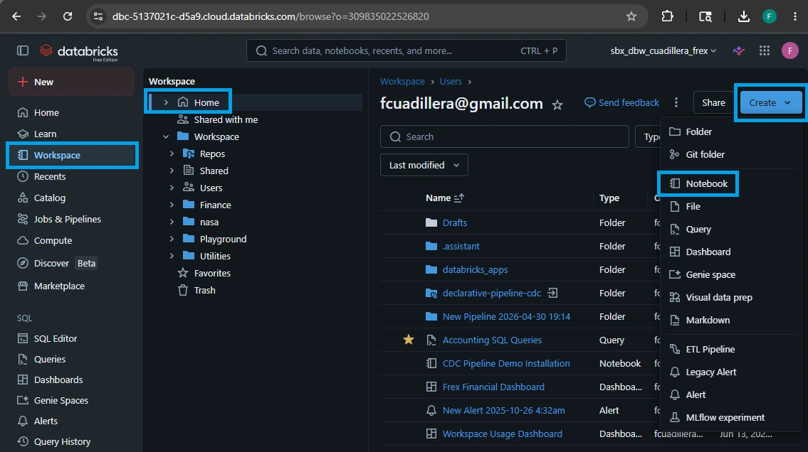
1.Open a Databricks Notebook:

Create a new notebook in your workspace and attach it to the Serverless compute.

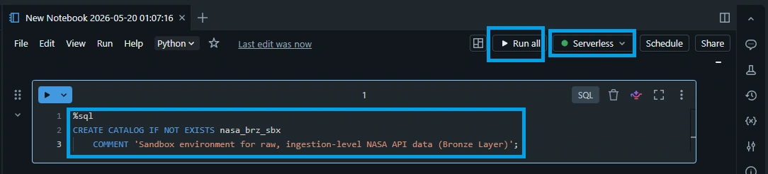
2.Execute the CREATE SQL command:

Copy and paste the following command into a code cell and run it:

This is the fastest method and can easily be integrated into your infrastructure setup scripts.

%sql
CREATE CATALOG IF NOT EXISTS nasa_brz_sbx
    COMMENT 'Sandbox environment for raw, ingestion-level NASA API data (Bronze Layer)';

Method 2: The Databricks UI Way (Catalog Explorer)

If you prefer a visual click-through approach, follow these steps:

Click on Catalog (the storage icon) in the left-hand sidebar of your Databricks workspace.
At the top right of the Catalog Explorer pane, click the blue Create Catalog button.
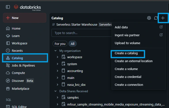
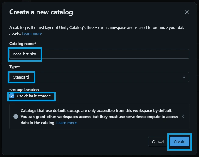
In the slide-out menu, configure the following:
- Catalog Name: Type nasa_brz_sbx.
- Type: Select Standard (unless you are linking an external data share via Delta Sharing).
(Optional) Storage Location: If your organization requires specific cloud storage buckets for sandboxes, paste the S3 or ADLS Gen2 path in the external location box. If left blank, it defaults to your metastore's root storage.
Click Create.

Your new nasa_brz_sbx catalog is now fully live and ready for you to create schemas (like nasa_brz_sbx.apod or nasa_brz_sbx.mars_rovers) to store your API ingestions!

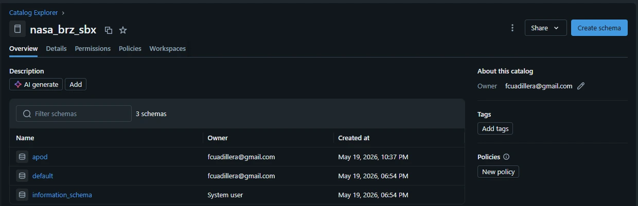
5.2. Schema

Now that you have your top-level nasa_brz_sbx catalog ready, the next step in the Unity Catalog hierarchy is creating a Schema (historically called a database in legacy Hive environments).

Creating the apod schema establishes a dedicated workspace folder inside your catalog to house all the raw tables, views, and volumes specifically tied to the Astronomy Picture of the Day API data.

5.2.1. The Three-Tier Namespace Reminder

By creating this schema, you are completing the second tier of Databricks' asset tracking system: nasa_brz_sbx (Catalog) ➔ apod (Schema) ➔ your_table_name (Table)

5.2.2. Step-by-Step Guide: Creating the Schema

You will need CREATE SCHEMA privileges on the nasa_brz_sbx catalog to run these commands. Just like the catalog setup, you can do this via SQL or the UI explorer.

Method 1: The SQL Notebook Way (Recommended)

%sql
CREATE SCHEMA IF NOT EXISTS apod
COMMENT 'Contains raw ingested data payloads from the NASA Astronomy Picture of the Day API';

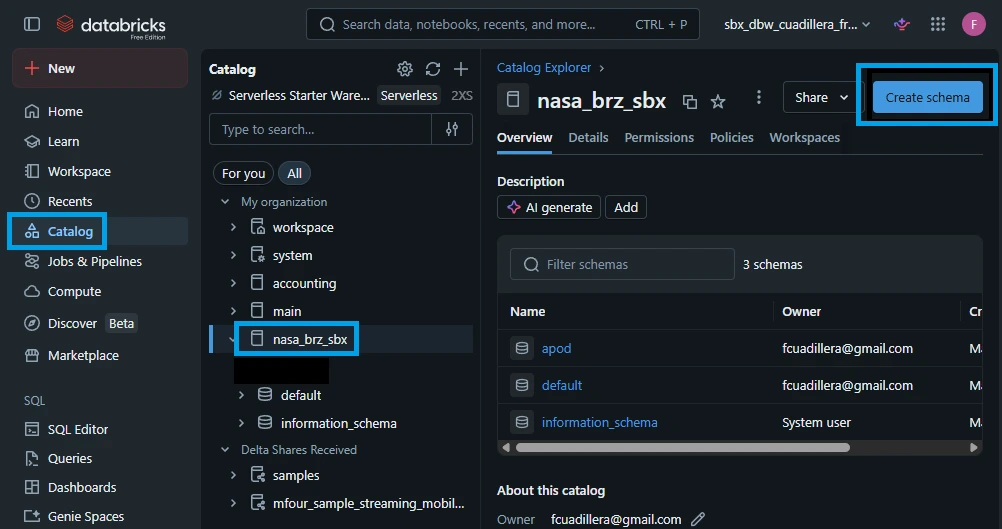
Method 2: The Databricks UI Way (Catalog Explorer)

Click on Catalog in the left-hand sidebar of your Databricks workspace.
In the left navigation tree of the Catalog Explorer, click on your catalog: nasa_brz_sbx.
In the main pane, look to the top right and click the blue Create Schema button.
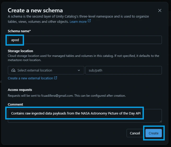
Fill in the schema details:
- Schema Name: Enter apod.
- Comment: "Contains raw ingested data payloads from the NASA Astronomy Picture of the Day API"
- (Optional) Storage Location: Leave blank to inherit the catalog’s root path, or specify an isolated storage path if your bronze layer requires explicit bucket routing.
Click Create.

Any notebooks or data pipelines can now target nasa_brz_sbx.apod to build and populate landing tables.

5.3. Volume

In Unity Catalog, a Volume is a critical feature for Medallion Architectures. While tables are great for structured rows, a Volume is a managed gateway to cloud object storage designed specifically for unstructured or semi-structured raw files—like the raw JSON payloads you get back from the NASA API.

By creating the astronomy_pictures volume, you are building a landing zone where your ingestion scripts can drop raw JSON text files before parsing them into tables.

5.3.1. Understanding the Volume Path

Unity Catalog automatically maps managed volumes to a deterministic POSIX-like file path pattern across your workspace: /Volumes/<catalog>/<schema>/<volume>

Because this is a Managed Volume, Databricks will automatically handle the underlying cloud storage allocation (S3 or ADLS Gen2) seamlessly behind the scenes. You don't have to manage storage IAM roles or mount paths; you can write to it just like a local directory folder.

5.3.2. Step-by-Step Guide: Creating the Volume

You will need CREATE VOLUME privileges on the nasa_brz_sbx.apod schema to execute these steps.

Method 1: The SQL Notebook Way (Recommended)

%sql
CREATE VOLUME IF NOT EXISTS astronomy_pictures
COMMENT 'Raw landing zone directory for JSON files pulled from NASA APOD API';

Method 2: The Databricks UI Way

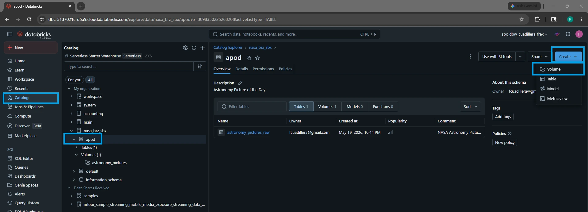
Open Catalog Explorer from your left sidebar.
Drill down into nasa_brz_sbx ➔ apod.
Click the Create button in the top right corner of the schema window and select Create Volume.
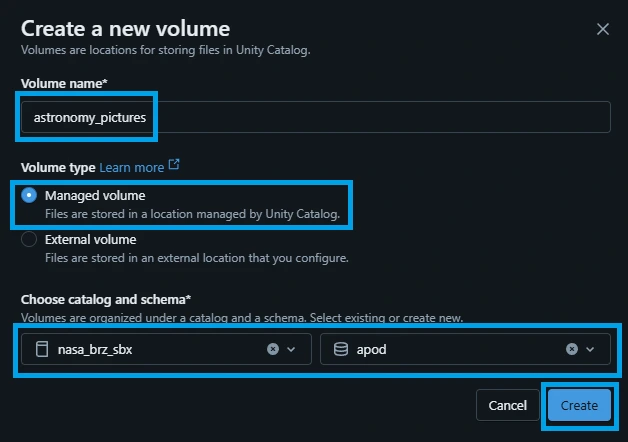
Configure the settings:
- Volume Name: astronomy_pictures
- Volume Type: Select Managed (this will automatically route files to the default schema location).
- Comment: Add a description (e.g., "Raw landing folder for APOD JSON partitions").
Click Create.

5.4. Tables

Now that your raw JSON storage volume is set up, the final step in your Bronze sandbox layer architecture is creating the structured Delta table: nasa_brz_sbx.apod.astronomy_pictures_raw.

Because this sits in the Bronze layer of the Medallion Architecture, our goal is to map the schema cleanly to the incoming NASA API payload attributes while keeping the data relatively raw. This ensures downstream Silver and Gold layer pipelines have a reliable foundation to query from.

5.4.1. Column Data Type Mapping

Based on the official NASA APOD documentation, all of these fields return as strings in the raw JSON response. However, we can optimize the table structure right away by enforcing proper data types (like using a real DATE type for the photo date) while leaving everything else as flexible strings.

Here is the data blueprint for your raw landing table:

Column Name	Data Type	Description
date	DATE	The day the astronomy picture was featured (Primary key logic)
title	STRING	The title assigned to the image/video
explanation	STRING	The deep-dive descriptive text written by an astronomer
url	STRING	Direct web link to the standard resolution media asset
hdurl	STRING	Direct web link to the high-definition version (if applicable)
media_type	STRING	Identifies if the asset is an image, video, etc.
copyright	STRING	The name of the photographer or institution holding rights
service_version	STRING	The internal NASA API version used to serve the request

5.4.1. Step-by-Step Guide: Creating the Table

You can execute this setup directly in your Databricks SQL notebook.

Because we want this table to perform optimally as it scales over time, we will explicitly configure it as a Delta Lake table and add an optimization setting.

Why the TBLPROPERTIES Matter for This Table

When you are loading small API files incrementally (like running a daily Cron job that appends one row or a small batch of rows from the NASA API), Delta tables can suffer from a phenomenon known as the "Small File Problem".

By adding 'delta.autoOptimize.optimizeWrite' = 'true' and 'delta.autoOptimize.autoCompact' = 'true', Databricks automatically handles file layouts in the background, consolidating data into larger, clean transactional chunks so your downstream queries remain incredibly fast.

Your full hierarchy is now officially complete:

nasa_brz_sbx (Catalog) ➔ apod (Schema) ➔ astronomy_pictures_raw (Table)

1.Target your target database context:

Open your Databricks notebook and ensure your engine session is locked into the correct apod schema:

%sql
CREATE TABLE IF NOT EXISTS astronomy_pictures_raw (
	date DATE COMMENT 'Date of the astronomy picture (YYYY-MM-DD)',
	title STRING COMMENT 'Title of the picture',
	explanation STRING COMMENT 'Detailed explanation written by 		       professional astronomers',
	url STRING COMMENT 'Standard resolution image or video player URL',
	hdurl STRING COMMENT 'High-definition image URL (null for videos)',
	media_type STRING COMMENT 'Type of media asset (e.g., image, video)',
	copyright STRING COMMENT 'Copyright holder information',
	service_version STRING COMMENT 'APOD API system version'
)
USING DELTA
TBLPROPERTIES (
	'delta.autoOptimize.optimizeWrite' = 'true',
	'delta.autoOptimize.autoCompact' = 'true'
)
COMMENT 'Bronze layer storage holding structured raw history logs from the NASA APOD API';

Confirm that Unity Catalog has successfully registered the structure and table properties inside the catalog layout:

%sql
SHOW TABLES; -- Confirm table is visible
DESCRIBE TABLE EXTENDED astronomy_pictures_raw; -- Review column metadata configurations

6. Building the Scheduled API Ingestion Job (API → Landing)

Our objective is simple: establish an ingestion pipeline that moves data from the NASA API directly into our Landing Zone (the Databricks Volume we created earlier). To achieve this with clean enterprise governance, we must first build out an organized directory hierarchy within our Databricks Workspace to isolate our code by domain, and then deploy our dedicated ingestion notebook.

6.1. Workspace Directory & Notebook Setup

Following corporate infrastructure standards, workspaces should be structured logically by Business Domain and Use Case. This prevents environment clutter, keeps repositories isolated across multiple data engineering squads, and prepares your codebase for complex scale-outs (like adding shared libraries or binaries folders later on).

For our specific use case, our notebook naming layout uses a professional, self-documenting prefix system: nbk_ (Notebook) ➔ ingest_ (Action) ➔ nasa_ (Domain) ➔ apod_ (Use Case) ➔ landing (Target Zone)

By applying your strategy, your workspace path will ultimately scale out to look like an enterprise layout:

/Workspace
  └── nasa/                      <-- Business Domain
       └── apod/                 <-- Use Case / Endpoint
            ├── libraries/       <-- (Optional generic helper utilities)
            ├── binaries/        <-- (Optional configuration files/jars)
            └── nbk_ingest_nasa_apod_landing  <-- Ingestion Script

6.2. Create the Workspace Directories

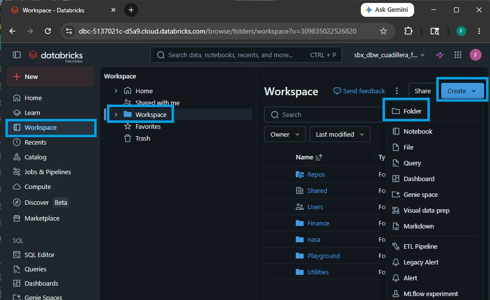
1.Navigate to Workspace Root:

On the left sidebar of your Databricks environment, click on the Workspace icon. Click the arrow to expand the /Workspace root directory folder.

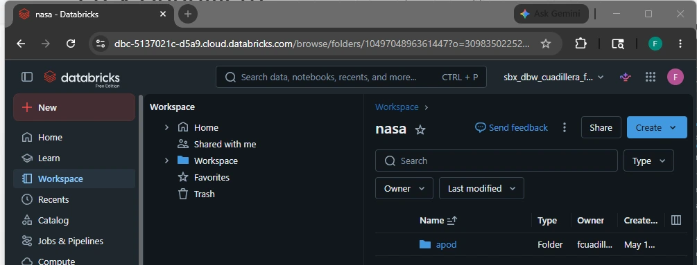
2.Create the Domain Folder ('nasa'):

Right-click on the main Workspace heading (or click the three vertical dots next to it), select Create ➔ Folder. Name this folder exactly nasa and press Enter.

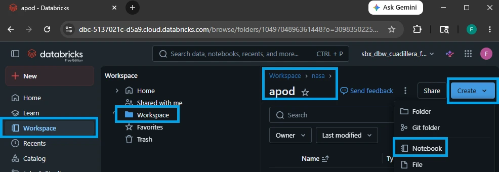
3.Create the Use Case Folder ('apod'):

Right-click directly on your newly created nasa folder, select Create ➔ Folder. Name this nested directory apod and press Enter. Your full directory hierarchy path is now officially established as /Workspace/nasa/apod/.

6.3. Instantiate the Ingestion Notebook Landing

Right-click directly on your newly created apod folder.
Select Create ➔ Notebook.
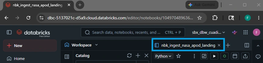
A blank notebook will open. At the top of the screen, click on the default generated name to rename it.
Set the name exactly to: nbk_ingest_nasa_apod_landing
Ensure the default language dropdown menu (located right next to the notebook title) is set to Python.

6.4. Writing the code for the ingestion landing notebook

Cell #1: Fetch NASA APOD data and insert into table

import requests
import json

# Get date parameter (defaults to today)
date_param = dbutils.widgets.get('date')
print(f"Fetching APOD data for date: {date_param}")

# NASA APOD API configuration
API_KEY = "YOUR_API_KEY"
API_URL =f"https://api.nasa.gov/planetary/apod?api_key={API_KEY}&date={date_param}"

# Volume path configuration
BASE_VOLUME_PATH ="/Volumes/nasa_brz_sbx/apod/astronomy_pictures"
partition_path =f"{BASE_VOLUME_PATH}/date={date_param}"
json_file_path =f"{partition_path}/apod_{date_param}.json"
jsonl_file_path =f"{partition_path}/apod_{date_param}.jsonl"

try:
	# Fetch data from NASA APOD API
	print(f"Calling API: {API_URL}")    
	response = requests.get(API_URL, timeout=30)    
	response.raise_for_status()

	# Parse JSON response    
	apod_data = response.json()
	print(f"Successfully retrieved APOD data: {apod_data.get('title', 'No title')}")

	# Create partition directory if it doesn't exist using dbutils
	try:        
		dbutils.fs.mkdirs(partition_path)
		print(f"Created/verified partition directory: {partition_path}")
	except:
		# Directory might already exist
		pass

	# Save as pretty-printed JSON using dbutils.fs    
	json_content = json.dumps(apod_data, indent=2)    	
	dbutils.fs.put(json_file_path, json_content, overwrite=True)
	print(f"✓ Saved JSON file: {json_file_path}")
	
	# Save as single-line JSONL using dbutils.fs    
	jsonl_content = json.dumps(apod_data) +'\n'  			
	dbutils.fs.put(jsonl_file_path, jsonl_content, overwrite=True)
	print(f"✓ Saved JSONL file: {jsonl_file_path}")
	
	print(f"\n✓ SUCCESS: APOD data for {date_param} saved to volume")
	print(f"JSON size: {len(json_content)} bytes")

except requests.exceptions.RequestException as e:
	print(f"ERROR: API request failed - {str(e)}")
	raise
except Exception as e:
	print(f"ERROR: Unexpected error - {str(e)}")
	raise

Technical Code Breakdown

1. Dynamic Orchestration & Parameterization

Instead of hardcoding a date, this script uses Databricks Workspace widgets to make the notebook completely dynamic.

date_param = dbutils.widgets.get('date')

dbutils.widgets.get('date'): This is the magic line for scheduling. When this notebook is eventually plugged into a Databricks Job, the orchestration scheduler will automatically pass a date parameter right here (e.g., passing today's date for daily runs, or a past date for historical backfilling).

2. API Communication & Security Guardrails

The script targets the NASA Astronomy Picture of the Day endpoint using your personal token.

response = requests.get(API_URL, timeout=30)
response.raise_for_status()

Network Timeout Protection: Setting timeout=30 is an excellent production practice. If NASA’s servers hang, your script will gracefully time out after 30 seconds rather than running indefinitely and wasting expensive cluster compute hours.
raise_for_status(): If the API returns a bad HTTP status code (like a 401 Unauthorized due to an expired key or a 429 Too Many Requests due to hitting rate limits), this built-in method intercepts it instantly and raises an error, ensuring the script fails fast instead of continuing with blank data.

3. Storage Routing & File System Utilities (dbutils.fs)

This section maps your data directly to the Unity Catalog Volume architecture we set up earlier.

BASE_VOLUME_PATH = "/Volumes/nasa_brz_sbx/apod/astronomy_pictures"
partition_path = f"{BASE_VOLUME_PATH}/date={date_param}"

Hive Partitioning Alignment: By constructing the folder string as /date=YYYY-MM-DD, it creates standard Hive/Spark storage partitions dynamically inside the managed volume.
dbutils.fs.mkdirs & dbutils.fs.put: Instead of using Python's native os and file context managers (open()), the code utilizes Databricks' optimized file system utilities (dbutils.fs). This ensures that file writes communicate natively and smoothly with your cloud object storage layer underneath the volume wrapper.

4. Dual-Format Landing Strategy (The "Why")

The most interesting architectural choice in this script is that it saves the exact same data payload into two different formats simultaneously inside your landing zone:

json_file_path = f"{partition_path}/apod_{date_param}.json"   # Pretty-printed
jsonl_file_path = f"{partition_path}/apod_{date_param}.jsonl" # Single-line JSONL

File Asset	Format	Why It Is There
.json	Pretty-Printed (Indented tabs)	Human Readability: If a data engineer or business analyst browses the Catalog Explorer and clicks on this file, it will be perfectly indented and incredibly easy to read and audit manually.
.jsonl	JSON Lines (Flat single-line + \n)	Machine Optimizations: Apache Spark handles multi-line JSON files poorly unless explicitly told to do so (which kills read performance). By flattening the payload into a single-line JSONL format with a newline breaker, Spark can read this file infinitely faster when loading data downstream into your final Delta table.

5. Global Error Handling

The script is safely wrapped inside a robust try-except block:

requests.exceptions.RequestException: Catches web-specific network errors (like DNS failures or bad HTTP states) and logs them clearly.
Exception as e: Catches unexpected bugs (like data parsing issues or file writing errors).
raise: By including raise at the end of both exception blocks, the script guarantees that if an error occurs, the notebook will throw a hard failure. This tells the automated Databricks Workflow engine to alert your data team that the pipeline broke, rather than quietly pretending everything succeeded.

Cell #2: Verify successful insertion

# Verify files exist and read them back
date_param = dbutils.widgets.get('date')
BASE_VOLUME_PATH ="/Volumes/nasa_brz_sbx/apod/astronomy_pictures"
partition_path =f"{BASE_VOLUME_PATH}/date={date_param}"
json_file_path =f"{partition_path}/apod_{date_param}.json"
jsonl_file_path =f"{partition_path}/apod_{date_param}.jsonl"

print(f"Verifying files for date: {date_param}\n")

# Check JSON file using dbutils.fs
try:    
	file_info = dbutils.fs.ls(json_file_path)    
	file_size = file_info[0].size
	print(f"✓ JSON file exists: {json_file_path}")
	print(f"  Size: {file_size:,} bytes")
	
	# Read and display a sample    
	content = dbutils.fs.head(json_file_path, 100000)  # Read up to 100KB    		
	data = json.loads(content)
	print(f"  Title: {data.get('title')}")
	print(f"  Media type: {data.get('media_type')}")
	print(f"  Copyright: {data.get('copyright', 'N/A')}")
except Exception as e:
	print(f"✗ JSON file not found or error reading: {json_file_path}")
	print(f"  Error: {str(e)}")

print()

# Check JSONL file using dbutils.fs
try:    
	file_info = dbutils.fs.ls(jsonl_file_path)    
	file_size = file_info[0].size
	print(f"✓ JSONL file exists: {jsonl_file_path}")
	print(f"  Size: {file_size:,} bytes")
except Exception as e:
	print(f"✗ JSONL file not found: {jsonl_file_path}")
	print(f"  Error: {str(e)}")

print(f"\n✓ All files verified successfully for {date_param}")

Here is the high-level explanation for Cell 2:

This cell acts as a quality assurance (QA) checkpoint to verify that the files you just generated in Cell 1 actually exist in your Volume and aren't corrupted.

Reconstructs Paths: It grabs the exact same date parameter and rebuilds the path strings to locate your .json and .jsonl files.
Verifies the Data Log (.json):
- Uses dbutils.fs.ls to make sure the pretty-printed JSON file exists and prints its file size.
- Uses dbutils.fs.head to read the file content directly, parsing and printing a quick sample preview (Title, Media type, Copyright) right in the notebook console to prove the payload is valid.
Verifies the Spark-Ready Log (.jsonl):
- Checks for the presence of your flat JSONL file to ensure the downstream ingestion table script has its source file ready to go.

If either file is missing or unreadable, the script catches the failure gracefully and prints an explicit error message instead of crashing silently.

6.5. Creating ingestion landing job

Here is how to create and schedule your automated pipeline job in Databricks to pull the NASA APOD data every morning.

NASA's main offices operate on US Eastern Time (ET). Scheduling your job for 8:00 AM Eastern Time ensures you catch the daily update right as it goes live.

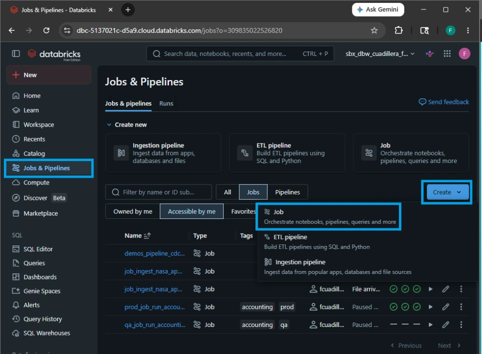
1.Navigate to Jobs & Pipelines:

On the left-hand navigation sidebar in Databricks, click on the Jobs & Pipelines. Click the blue Create Job button in the top right corner.

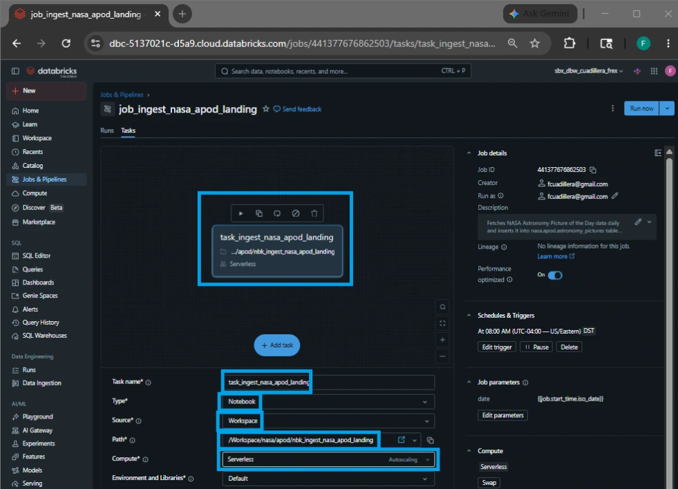
2.Configure the Notebook Task:

A task configuration window will open. Set up the following parameters:

Task name: task_ingest_nasa_apod_landing
Type: Notebook.
Source: Workspace.
Path: /Workspace/nasa/apod/nbk_ingest_nasa_apod_landing.
Compute: Serverless
Environment and libraries: default

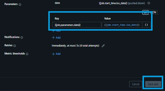
3.Add the Dynamic Date Parameter:

Under the Parameters section on the right side of the task card, click Add. This is where we feed the widget we built inside the script:

Key: {{job.parameters.date}}
Value: {{job.start_time.iso_date}} (This is a dynamic Databricks system variable that automatically calculates and inserts the current execution date in YYYY-MM-DD format every time the job runs).

Click Create task.

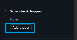
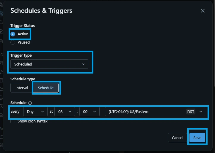
4.Set the Schedule (8:00 AM Eastern):

On the right-hand panel of the main Job page, locate the Job details box and click Add trigger.

Trigger Status: Active
Trigger type: Select Scheduled.
Schedule type: Schedule
Schedule: Set to Every day at 08:00.
Time zone: Search for and select "(UTC-04:00) US/Eastern" to lock it directly to NASA's Eastern Time zone.

Click Save.

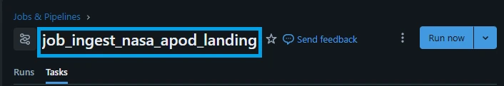
Pro-Tip: Remember to change the top-left title of your job from "Untitled Job" to something clear and recognizable, like job_ingest_nasa_apod_landing.

5.Rename the job:

Double click the top-left title of your job from "New Job" to: job_ingest_nasa_apod_landing.

7. Building the File Arrival Trigger Raw Ingestion Job (Landing → Raw Table)

Now that our landing pipeline is automatically dropping files into our volume at 8:00 AM Eastern Time, we need to handle the next phase of the Medallion Architecture: moving data from the landing directory into a structured structured table (Landing ➔ Raw Table).

Instead of scheduling this second step on a time clock and guessing when the files will finish downloading, we will configure an event-driven File Arrival Trigger. Databricks will constantly monitor our storage volume and wake up our processing pipeline the exact moment a new .jsonl file hits the storage layer.

7.1. Workspace Notebook Setup

To maintain an organized corporate folder structure, we will place our data processing notebook right next to our landing script inside our /Workspace/nasa/apod/ directory.

Following our strict engineering naming conventions:

nbk_ (Notebook) ➔ ingest_ (Action) ➔ nasa_ (Domain) ➔ apod_ (Use Case) ➔ raw (Target Zone)

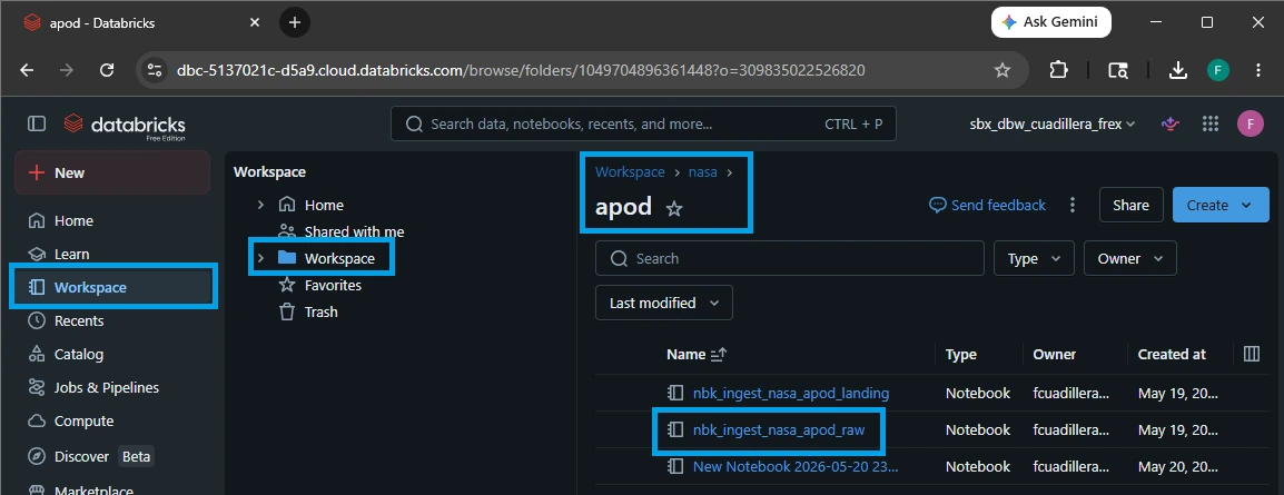
7.2. Instantiate the Ingestion Notebook Raw

Open the Workspace tab on the left sidebar and open /Workspace/nasa/apod/.
Right-click on the apod folder, select Create ➔ Notebook.
Name the notebook exactly: nbk_ingest_nasa_apod_raw
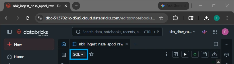
Set the default language dropdown to SQL

7.3. Writing the code for the ingestion raw notebook

Cell #1: Create target table if not exists

CREATE TABLE IF NOT EXISTS nasa_brz_sbx.apod.astronomy_pictures_raw (
		date DATE COMMENT 'Date of the astronomy picture', 
		title STRING COMMENT 'Title of the picture',
		explanation STRING COMMENT 'Detailed explanation of the astronomical phenomenon',
		url STRING COMMENT 'URL of the standard resolution image',  
	hdurl STRING COMMENT 'URL of the high-definition image',  
		media_type STRING COMMENT 'Type of media (image, video, etc.)',  	
	copyright STRING COMMENT 'Copyright holder of the image',  
		    service_version STRING COMMENT 'APOD API service version'
)
COMMENT 'NASA Astronomy Picture of the Day (APOD) raw data from volume'

Cell #2: Read new data from volume and filter existing dates

-- Read all JSONL files from volume (partitioned by date)
CREATE OR REPLACE TEMP VIEW new_apod_data AS
SELECT
	CAST(date AS DATE) as date,
	title,
	explanation,
	url,
	hdurl,
	media_type,
	copyright,
	service_version
FROM read_files(
	'/Volumes/nasa_brz_sbx/apod/astronomy_pictures/date=*/apod_*.jsonl',
	format => 'json'
)
WHERE date NOT IN (
	SELECT DISTINCT date
	FROM nasa_brz_sbx.apod.astronomy_pictures_raw
)

Cell #3: Merge new records into target table

MERGE INTO nasa_brz_sbx.apod.astronomy_pictures_raw AS target
USING new_apod_data AS source
ON target.date = source.date
WHEN NOT MATCHED THEN
INSERT (
	date,
	title,
	explanation,
	url,
	hdurl,
	media_type,
	copyright,
	service_version
)
VALUES (
	source.date,
	source.title,
	source.explanation,
	source.url,
	source.hdurl,
	source.media_type,
	source.copyright,
	source.service_version
)

Cell #4: Show newly processed dates in this run

-- Show which dates were processed in this run.
SELECT
	date,
	title,
	media_type
FROM new_apod_data
ORDER BYdateDESC

Cell #5: Show ingestion summary

-- Show summary of ingested data
SELECT
	COUNT(*) as total_records,
	MIN(date) as earliest_date,
	MAX(date) as latest_date,
	COUNT(DISTINCTdate) as unique_dates
FROM nasa_brz_sbx.apod.astronomy_pictures_raw

Technical Code Breakdown

Inside your nbk_ingest_nasa_apod_raw notebook, the data pipeline runs in three clear, robust SQL phases designed to process files idempotently (meaning it guarantees zero data duplication even if the job runs multiple times on the same data).

1. Schema Enforcement

The notebook kicks off by ensuring your permanent Delta lake table target exists:

CREATE TABLE IF NOT EXISTS nasa_brz_sbx.apod.astronomy_pictures_raw (
  date DATE COMMENT 'Date of the astronomy picture',
  title STRING COMMENT 'Title of the picture',
  ...
)

This guarantees the data pipeline won't crash on its first-ever execution run if the base table hasn't been built yet.

2. Wildcard Directory Scanning & De-duplication

Next, instead of hardcoding file targets, the notebook uses the highly efficient read_files function to dynamically crawl through every directory partition inside your volume. It filters out files that have already been imported using an anti-join subquery:

CREATE OR REPLACE TEMP VIEW new_apod_data AS
SELECT CAST(date AS DATE) as date, title, explanation, url, hdurl, media_type, copyright, service_version
FROM read_files(
  '/Volumes/nasa_brz_sbx/apod/astronomy_pictures/date=*/apod_*.jsonl',
  format => 'json'
)
WHERE date NOT IN (SELECT DISTINCT date FROM nasa_brz_sbx.apod.astronomy_pictures_raw)

3. The Idempotent Upsert (MERGE)

Finally, it runs a transactional MERGE INTO statement to safely append the newly discovered dates into your core asset table:

MERGE INTO nasa_brz_sbx.apod.astronomy_pictures_raw AS target
USING new_apod_data AS source
ON target.date = source.date
WHEN NOT MATCHED THEN
  INSERT (date, title, explanation, url, hdurl, media_type, copyright, service_version)
  VALUES (source.date, source.title, source.explanation, source.url, source.hdurl, source.media_type, source.copyright, source.service_version)

By explicitly matching on target.date = source.date and executing ONLY WHEN NOT MATCHED THEN INSERT, this job is bulletproof. If you backfill historical months or drop multiple days of raw logs into the volume at once, this pipeline will catch them all, skip what it already has, and append only the net-new records.

4. Real-Time Run Auditing

This query acts as an active execution log, showing you exactly what the pipeline accomplished during its current run.

SELECT date, title, media_type
FROM new_apod_data
ORDER BY date DESC

Targeting the Transient Layer: By querying new_apod_data (the temporary view created in Cell #2) instead of the final physical table, you isolate only the files processed during this specific trigger event.
Immediate Content Visibility: Pulling the title and media_type allows engineers to quickly spot-check the incoming data directly from the notebook output console to ensure everything looks correct.
Chronological Sorting: Sorting by date DESC places the absolute newest records at the top of the interface, which is ideal for verifying daily automated runs.

5. Global Health & Aggregation Summary

This cell provides a bird's-eye view of your entire dataset's health. It looks past individual files to evaluate the overall state of your raw data warehouse asset.

SELECT 
  COUNT(*) as total_records,
  MIN(date) as earliest_date,
  MAX(date) as latest_date,
  COUNT(DISTINCT date) as unique_dates
FROM nasa_brz_sbx.apod.astronomy_pictures_raw

Data Volume Tracking (COUNT(*)): Monitors the total row count inside astronomy_pictures_raw to track database growth over time.

Timeline Boundary Auditing (MIN / MAX): Identifies the oldest and newest dates currently captured in your system. This is incredibly helpful during historical backfills to verify if your historical range matches your target window.

Integrity Validation (COUNT(DISTINCT date)): This is your primary quality control metric. Because the APOD API only publishes one record per day, your unique_dates count should always perfectly match your total_records count. If total_records is ever higher, it instantly alerts you that duplicate entries slipped past your primary MERGE defenses.

7.4. Creating the ingestion raw job

Unlike the landing pipeline which runs on a time-based schedule, this job relies on an event-driven architecture. It continuously listens to your Unity Catalog Volume and wakes up the moment a new file drops.

1.Create a New Job:

In the left-hand navigation sidebar of Databricks, click on the Jobs & Pipelines. Under the Jobs tab, click the blue Create Job button in the top right corner. Rename your job at the top-left of the screen to: "job_ingest_nasa_apod_raw"

2.Configure the Notebook Task:

A task configuration window will automatically slide open. Fill out the details exactly as follows:

Task name: task_ingest_nasa_apod_raw
Type: Notebook.
Source: Workspace.
Path: /Workspace/nasa/apod/nbk_ingest_nasa_apod_raw
Compute: Serverless
Parameters: Leave this completely blank

Click the blue Create task button.

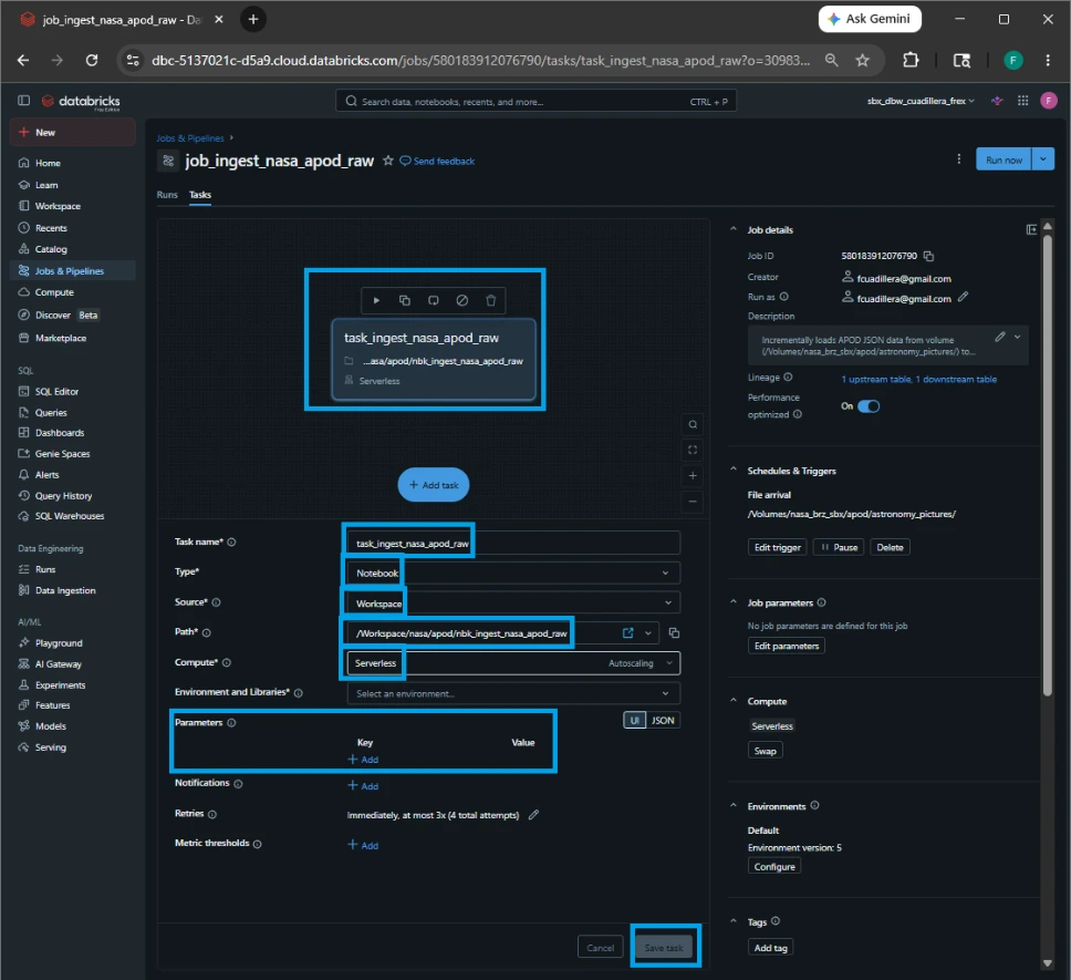
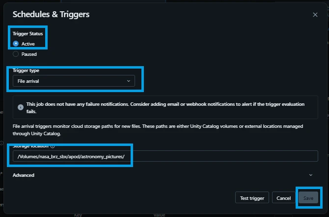
3.Configure the File Arrival Trigger:

Look over to the right-hand Job details configuration panel. Locate the Triggers section and click Add trigger.

Trigger Status: Active
Trigger type: File arrival
Storage location: /Volumes/nasa_brz_sbx/apod/astronomy_pictures/

Click Save.

Activating and Testing the Complete Pipeline

To bring your event-driven setup live, toggle the Status switch in the top right corner of the job page from Paused to Active.

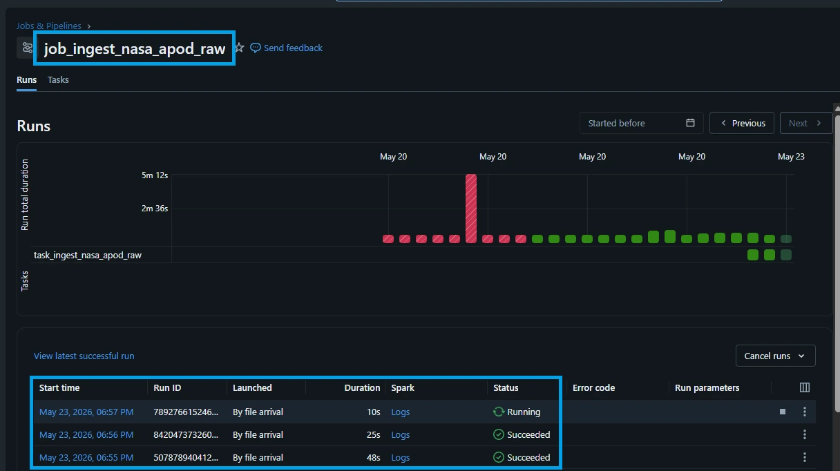
How the Pipeline Works End-to-End:

Every morning at 8:00 AM Eastern Time, job_ingest_nasa_apod_landing fires off on its schedule, downloads the data payload from NASA, and drops a new .jsonl file into /Volumes/nasa_brz_sbx/apod/astronomy_pictures/date=2026-05-23/.
The instant that file lands, Unity Catalog detects the file creation event and alerts the workflow manager.
Your new job_ingest_nasa_apod_raw automatically wakes up, executes task_ingest_nasa_apod_raw, runs the notebook's MERGE logic to cross-check dates, and commits the fresh data into your astronomy_pictures_raw table without a single second of manual intervention.

8. Backfilling Historical NASA APOD Data

Now that your event-driven pipeline is active, it will run perfectly moving forward. However, your astronomy_pictures_raw table will sit completely empty until the next 8:00 AM Eastern Time trigger fires.

To turn your empty table into a rich database right away, we can leverage the Backfill Feature in Databricks Jobs. Because we designed our landing notebook to accept a dynamic date parameter, we don't need to rewrite any code. We can simply instruct Databricks to spin up multiple parallel runs of our landing job, passing a different historical date to each run.

8.1. Running a Backfill Job

Follow these steps to retroactively load a window of past APOD records into your Bronze storage layer.

1.Open the Landing Job Workspace:

Navigate to the Jobs & Pipelines tab on the left sidebar of your Databricks environment. Under the Jobs tab, click on your landing job: job_ingest_nasa_apod_landing.

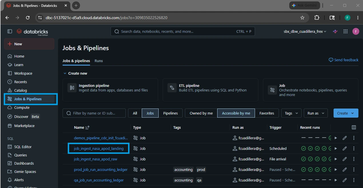
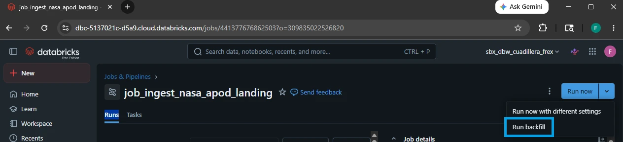
2.Locate the Run Now Dropdown:

In the top right corner of the job's overview page, look for the blue Run now button. Click the down arrow icon directly next to it and select Run backfill.

3.Open the Backfill Interface:

A configuration pane will appear. Instead of typing a single date parameter into the box, look at the bottom left of the window and click the link labeled Run a backfill.

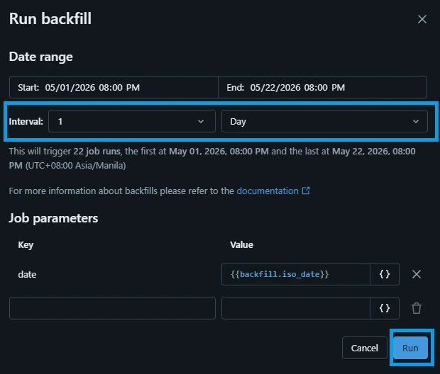
4.Configure the Backfill Window:

Set the parameters to define your historical timeline:

Time grain: Select Day (since the NASA APOD API updates once per day).
Start date: Pick your starting historical point (e.g., 2026-05-01).
End date: Set it to yesterday's date (e.g., 2026-05-22).

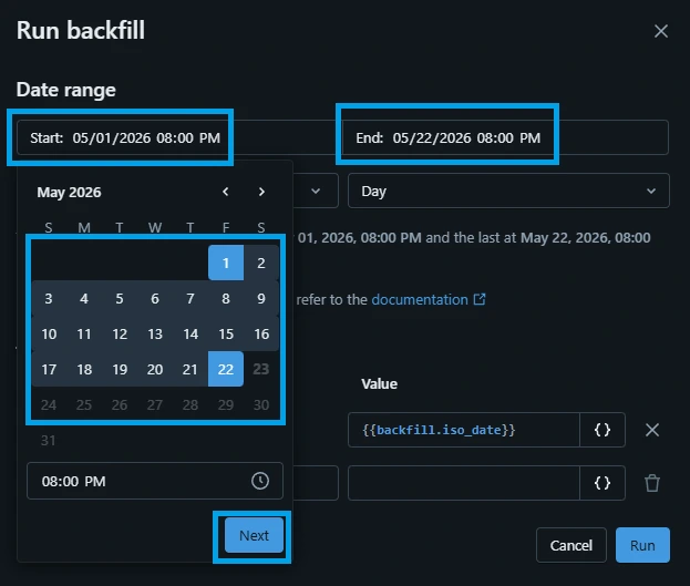
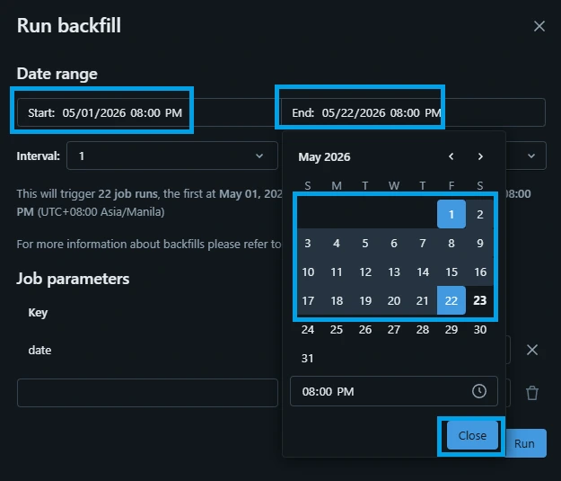
Click the Run button.

8.2. What Happens Behind the Scenes?

The moment you hit run, Databricks launches a visual matrix of parallel job tasks:

Mass Ingestion: The job_ingest_nasa_apod_landing workflow automatically clones itself for every single day in your chosen date range.
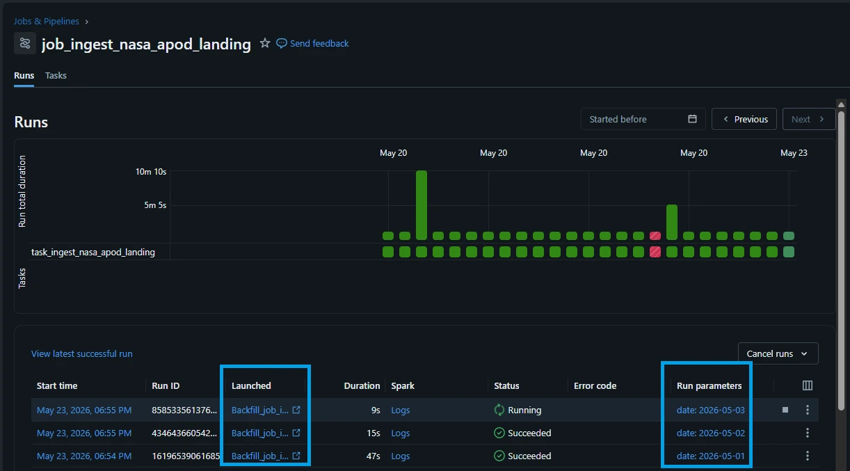
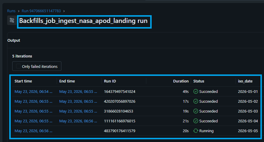
Automated Partitioning: Each parallel notebook landing task grabs its assigned date, downloads the target payload from NASA, and builds its own unique /date=YYYY-MM-DD/ subfolder inside your Unity Catalog Volume.
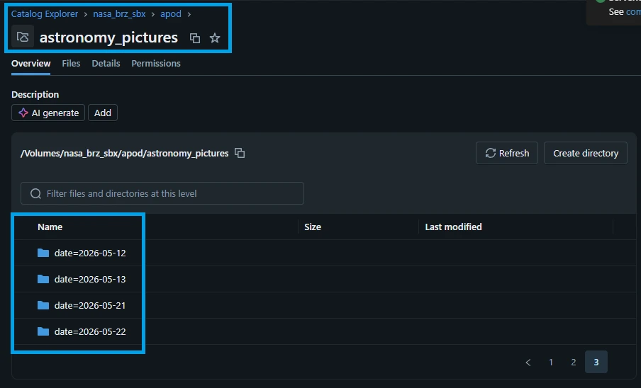
The Domino Effect: The second your storage volume registers those individual .jsonl file arrivals, your file arrival trigger—job_ingest_nasa_apod_raw—will instantly catch them, process the payloads through your SQL MERGE statement, and stack them cleanly into your permanent astronomy_pictures_raw table.

8. Validating Data & Monitoring Pipeline Health

An automated data pipeline is only as good as its visibility. Once your backfill completes and your daily ingestion schedules are live, you need a way to ensure data integrity and receive immediate notifications if a network glitch or API failure breaks the chain.

In this final section, we will cover how to easily audit your ingestion results using a quick SQL validation query, and how to configure Databricks Workflow Alerts to notify your team the instant a job fails.

8.1. Quick Data Validation with SQL

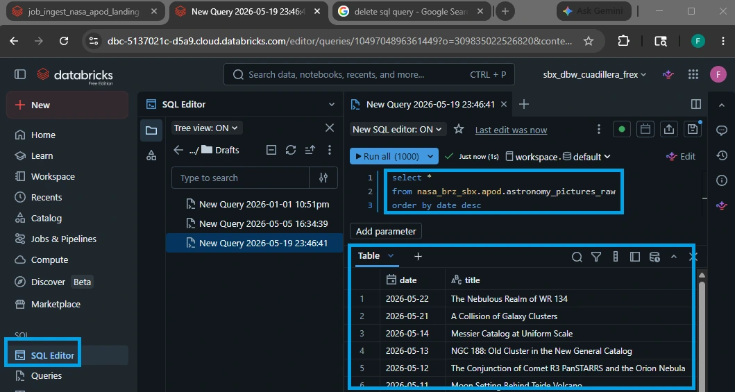
To verify that your incoming NASA API records are parsing correctly and landing safely inside your Delta Lake storage layer, you can run a simple, real-time validation query.

Open a Databricks SQL Editor or add a new cell to a notebook, and run the following query:

SELECT * FROM nasa_brz_sbx.apod.astronomy_pictures_raw 
ORDER BY date DESC;

8.3. What to Look For During Your Audit:

Chronological Alignment: Sorting by date DESC places the absolute newest records at the very top of your data preview grid, allowing you to instantly confirm if today's image successfully synced.
Payload Complete Cleanliness: Scan columns like title, url, and media_type. Ensure that fields aren’t shifted (e.g., descriptions accidentally leaking into the URL field) and that data styles are uniform.
Null Check Diagnostics: Ensure that hdurl is only empty when media_type is a video asset (as NASA rarely provides high-definition source streams for video player embeds).

8.4. Setting Up Production Job Health Alerts

You shouldn't have to manually check your tables every morning to see if your pipelines ran successfully. Instead, you can leverage the built-in Notifications and Alerts system in Databricks Workflows to monitor job statuses passively.

You can configure notifications for both your time-scheduled landing job (job_ingest_nasa_apod_landing) and your event-driven raw table job (job_ingest_nasa_apod_raw).

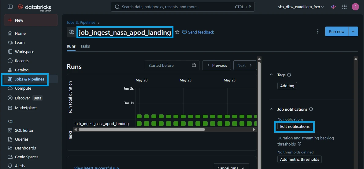
1.Open Your Job Configuration:

Navigate to the Jobs & Pipelines tab on your left sidebar, select your target job from the list, and look over at the right-hand Job details panel.

2.Access Notification Settings:

Locate the Notifications field inside the Job details card and click on Edit notifications (or the pencil icon).

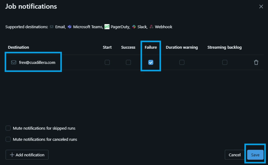
3.Configure Alert Destinations and Triggers:

A modal configuration window will appear. Configure your routing destinations here:

Email / Destination: Enter your personal work email, an engineering team distribution list, or a system webhook URL (such as a Microsoft Teams or Slack incoming webhook).
Triggers: Check the box next to Failure (Crucial: This triggers an alert the second a task encounters an unhandled API error or a cluster crash).

4.Save Your Alert Rule:

Click Save. Your automation workflow is now fully monitored.

9. Conclusion

Driven by a community push to eliminate high infrastructure costs and steep learning curves, building Databricks pipelines is now highly accessible. This supports Databricks’ core mission of data democratization: empowering everyone, regardless of technical background, with the basic skills to gather data and independently unlock insights.

#Data #DataEngineer #DataEngineering #Databricks #NASA

in Tech

# Technology